
Cindy’s in a major Omega campaign, Naomi’s back on the catwalk and Donatella broke the internet with her reunion of the ‘famous five’ for the Versace SS18 show. As the original supers stalk back into the spotlight, here’s our edit of the best models of all time.
Introduction by Autumn Whitefield-Madrano
If you were old enough to reach a newsagent counter in 1990, you’ll remember that cover: Naomi, Linda, Tatjana, Christy and Cindy, high-glam action figures clustered together, gazing at us on the front of January Vogue. Even those of us who fancied ourselves too lofty for supermodel daydreams were entranced by Peter Lindbergh’s black and white photo, elevated from the realm of fashion and approaching something closer to cinema. It was the image that kicked off the era of supermodel mania. If you weren’t old enough the first time round, you’ll definitely remember a certain Instagram-breaking moment last September – a similarly Amazonian line-up of Cindy, Claudia, Naomi, Carla and Helena, reunited on the Versace SS18 catwalk. The ‘supermodel’ has come full circle – quite literally in the case of these returning stars, whose stock has never been higher than now.
The original gang, a bit like the Spice Girls, had someone for everyone. Naomi Campbell: assertive, playful yet exquisite, the obvious icon not only for young black women, but for those who coveted her haughty ‘I’m worth it’ chutzpah. Linda Evangelista: chameleon-like with her ever-changing hair colour, yet always unmistakable, and admired for the gumption of saying she wouldn’t get out of bed for less than $10,000 a day. Christy Turlington, with her calm doe-eyed gaze and impossibly perfect features that looked carved from soapstone. Cindy Crawford and Tatjana Patitz, the smiling, can-do faces of athletic vigour on each side of the pond. That cover was shot more than a quarter of a century ago, yet ask most people to name a supermodel, and chances are at least one member of this quintet will roll instantly off the tongue.
Not that they were the first to be termed ‘supermodels’. The word has been bandied about since 1891, when painter Henry Stacy Marks rhapsodised about a certain variety of sitter: ‘The “super” model… goes in for theatrical effect; always has an expression of “Ha! Ha! More blood…”’ With each person dubbed a ‘supermodel’ over the 75 years it took for the term to take hold, the profession took form. To be a supermodel is to be an entity larger than that of fashion plate: Lisa Fonssagrives, a Swede widely considered to be the very first of the type, is perhaps known as such because she leveraged her modelling streak of the 40s into a fashion-design career. You also need to be instantly recognisable, to have a Cindy Crawford-mole USP, if you will: when Dorian Leigh – another candidate for the world’s first supermodel – met legendary editor Diana Vreeland, Mrs V told her, ‘Do not – do not do anything to those eyebrows!’ Perhaps it’s about celebrity (Twiggy prompted The New York Times’ first use of the word, in 1968), or an unshakeable self-belief (Janice Dickinson claimed she coined the term in 1979, which is patently untrue).
If the 1990 quintet were the first graduating class of modern supermodels, Kate Moss was its first rogue scholar. She seized the public eye in a singular fashion: she was unhealthily skinny, the story went, and then there was that whole ‘heroin chic’ thing. Plus, she didn’t care, or at least she didn’t look like she did. That deadpan expression, that flatness echoed by the broad planes of her face – teenage girls who couldn’t disguise that they cared desperately about boys, good grades and being liked were probably infuriated by her insouciance, consoling themselves by silently thinking, ‘She isn’t even that pretty.’
It’s this, I now see, that made her a supermodel. Kate Moss is no gargoyle; she doesn’t even qualify as jolie laide. But her face was the next logical step from the template that her supermodel elders had etched. Evangelista et al were jaw-droppingly beautiful, none of them dabbled in plebeian prettiness. Kate, with her much-mentioned (in model terms) shortness, ‘bandy’ legs and gappy smile, had the same magnetism and uniqueness they all share. Mere beauty isn’t what set them apart. To earn the ‘super’ prefix, a model doesn’t have to be the most beautiful model nor does she have to be the most commercially successful. She has to have that ineffable quality known as ‘It’, even as her It-ness is conferred upon a supermodel largely after her christening. She has to be comfortable with that, inhabit it and use it to her advantage. ‘There was nothing like these girls,’ says Sasha Charnin Morrison, who witnessed the rise of the supermodel during her 30-plus years in fashion publishing, including stints as fashion director at Harper’s Bazaar, Allure and Us Weekly. ‘When they said things like, “I don’t get out of bed for less than $10,000 a day,” that made complete sense. They were worth every penny.’
And they were, for a while. The predecessor to the model was the mannequin; models were referred to as ‘live mannequins’ before we settled upon our current term. A model’s job is to wear clothes, to be dressed, styled and passively done unto. The supermodels turned this on its head – the essence of feminism is the ability to have a choice, and these women were the ones doing the choosing. They were in control of their bodies, careers and the clothes they agreed to wear – and they sold them. It is less about possessing beauty and more about possessing a ‘look’– one that can shift depending on circumstance and styling, of course. A model asks that you look at her as a part of the whole – the fashion, the make-up, the hair, the mise-en-scène. A supermodel asks no such thing; she demands, and in doing so makes it clear that it is her essence that should remain indelible in your mind.
Which was, of course, their downfall. By 1998, Time had declared the death of the supermodel, with good reason. Moss walked for Alexander McQueen in spring 1997; a year and a half later, his showstopping Joan of Arc show featured relative nobodies. Designers wanted their creations to take centre stage, and magazine covers used actresses when they wanted recognition, and lesser-known models when they wanted the face of ‘relatability’ – the idea being that readers better project their own identity on to a blank canvas, unaccompanied by the overwhelming individuality of a Cindy or a Naomi.
Today’s supermodels may not have inherited their predecessors’ iconic status as models, but their DNA carries other imprints: business acumen (Cindy founded an empire on fitness videos before YouTube was a twinkle in Steve Chen’s eye), brand relationships, distinct yet pliant identities. While the originals were made into stars by endless press coverage, social media has allowed Gigi, Bella and Kendall to create stars of themselves. They aren’t at the mercy of the press for their image; they create their own personae, controlling what to reveal and what to conceal. With this ability to generate mystery, the new supermodel has mastered the catch-22 of It-ness, along with the business savvy that goes with the title. What remains to be seen is whether they will develop the quality that sees a quorum of the Vogue five working into their 50s – the ability to compel. When you look at Naomi Campbell lounging on a bed, gazing into the camera with a languid tease, you see light. Perhaps you envy her, but your deeper envy belongs to the photographer, able to watch her transcendence from behind the safety of the lens. You can’t tear your eyes away.
Scroll down for our best models ever hall of fame…
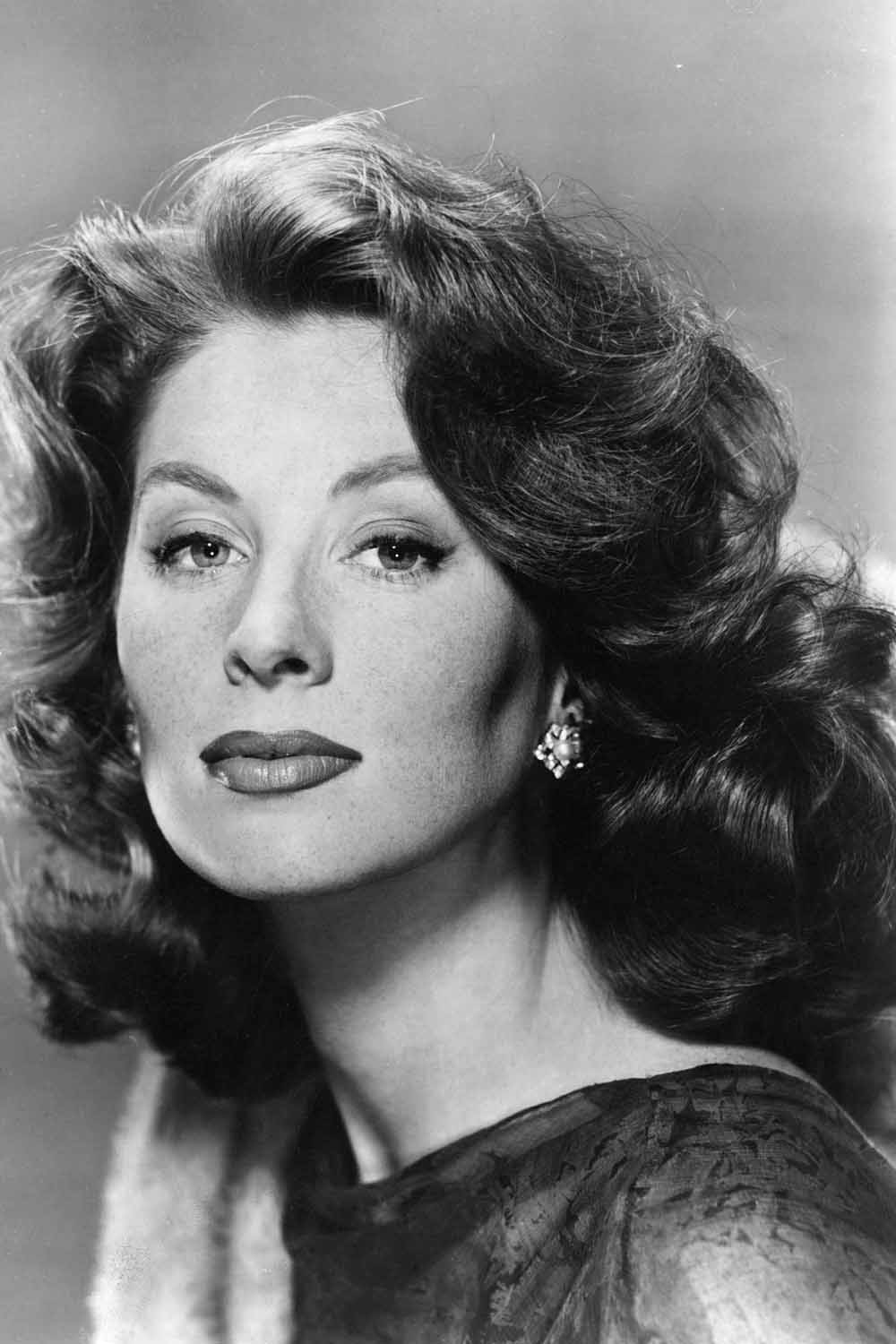
1. Suzy Parker
(Image credit: REX/Shutterstock)
Era: Late 1940s — early 1960s From: New York Her look: Freckly and flame-haired with an hourglass figure USP: A favourite muse of photographer Richard Avedon, her sister Dorian was a famous model, dubbed the ‘world’s first supermodel’. That was before the world met Suzy. She went on to eclipse her sis, becoming the first model to earn $100,000 per year and the only one to have an (unreleased) Beatles song named after her
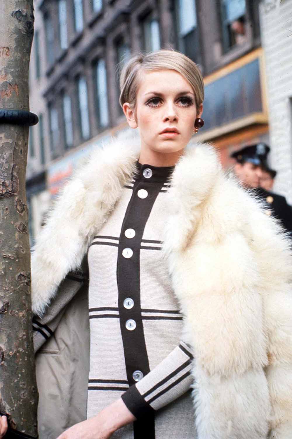
2. Twiggy (AKA Lesley Hornby)
(Image credit: REX/Shutterstock)
Era: 1960s From: Neasden, North-West London Her look: Bambi — after a few weeks of no dinner. Big eyes, spidery lashes and a skinny twig-like frame (hence the nickname). USP: Invented the Swinging Sixties — with a little help from the Beatles, Carnaby Street, et al. Discovered at 16 when she had her hair chopped off in hairdresser Leonard’s West End salon — a fashion journalist saw the pictures, and the rest is history.
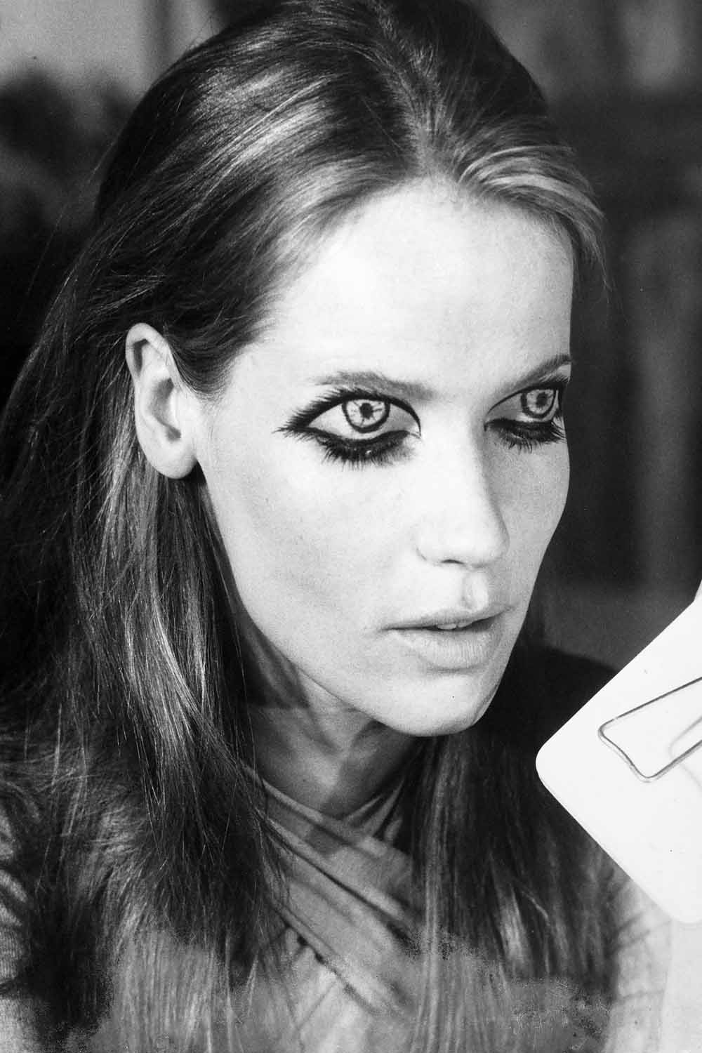
3. Veruschka
(Image credit: Alinari/REX/Shutterstock)
Era: 1960s From: Kaliningrad, Russia. Her look: A lionine mane of blonde hair and the kind of versatile face that could take any look — fake ‘eyes’ on her eyelids, being covered in gold leaf… You name it, she pulled it off USP: Her blue blood and fascinating family. Real name: Vera Gottliebe Anna Gräfin von Lehndorff-Steinort. Her mother was a Prussian countess and her father was a German count who was an active member of the Resistance — he was eventually executed for an assassination attempt on Adolf Hitler.
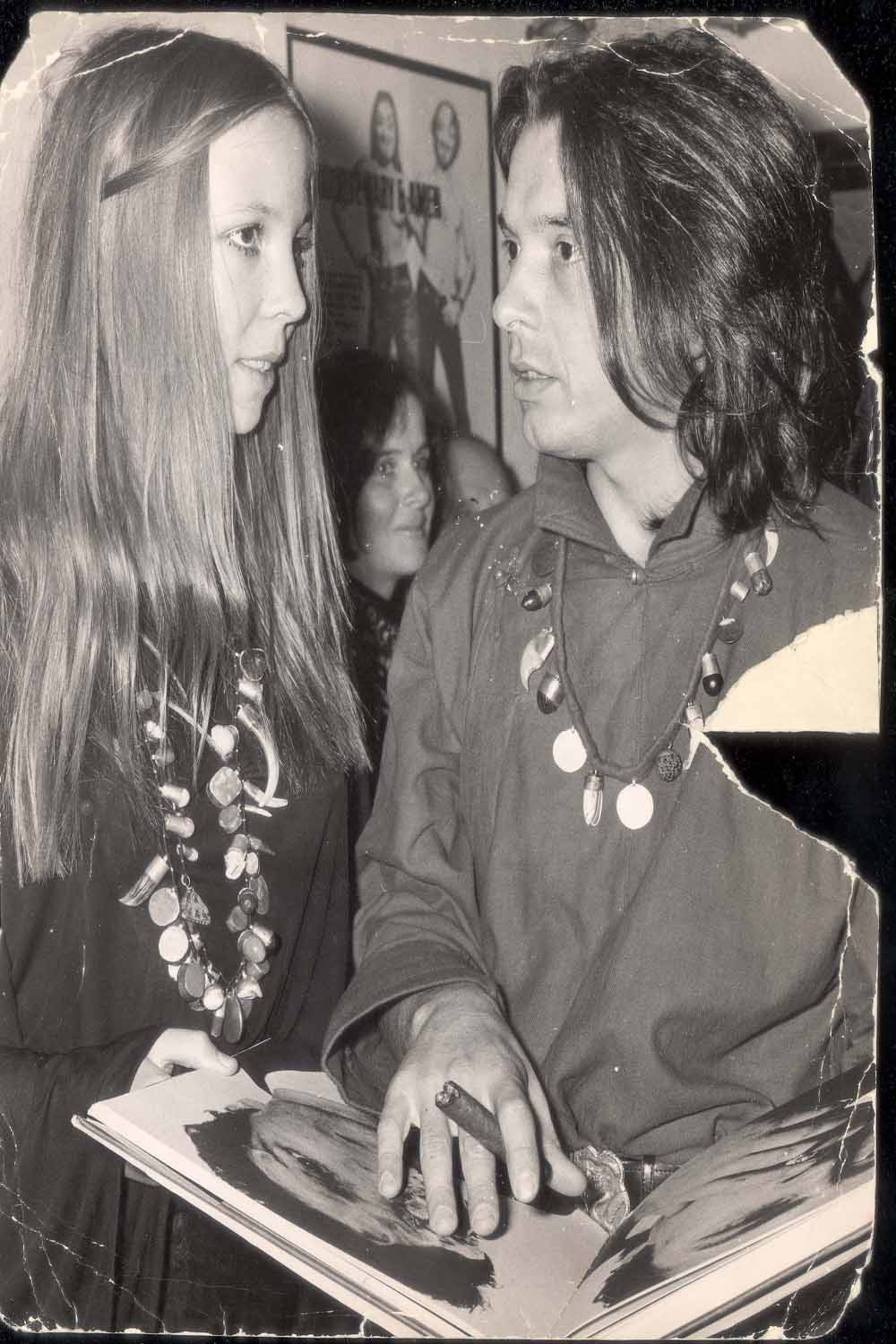
4. Penelope Tree
(Image credit: Daily Mail/REX/Shutterstock)
Era: 1960s From: UK Her look: Saucer eyes, spiky lashes and poker-straight hair. ‘An Egyptian Jimminy Cricket’ according to her then-boyfriend, cheeky chappie photographer David Bailey. USP: Super-connected socialite roots — brought up in the US, her mother was an American socialite descended from famous social activist Endicott Peabody. Her British MP dad threatened to sue if her first-ever photos (by legendary photographer Diane Arbus) were published.
5. Jean Shrimpton (AKA ‘The Shrimp’)
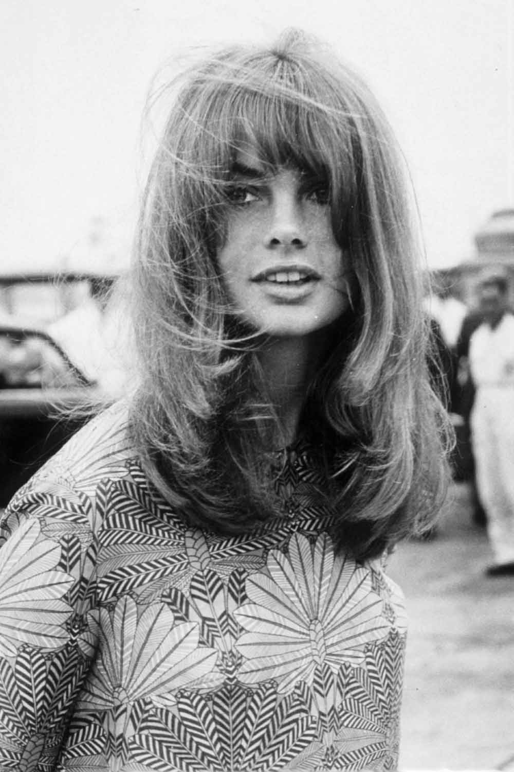
(Image credit: REX/Shutterstock)
Era: 1960s From: High Wycombe, Buckinghamshire Her look: Delicate, snub-nosed perfection USP: Yet another David Bailey conquest, she started her affair with him when he was still married to his first wife, who he divorced to be with Shrimpton. Described as having ‘the world’s most beautiful face’, everything she wore (even barely visible in a beauty campaign) was always a sell-out
6. Pat Cleveland
(Image credit: Evening Standar/REX/Shutterstock)
Era: 1960s-Present From: New York Her look: European-style beauty with a free-flowing mane of black hair USP: One of the most famous black models to break through fashion’s exclusionary policies of the 60s, she was named ‘the all-time superstar model’ by former US Vogue editor, André Leon Talley. Modelling for designers from Valentino to Yves Saint Laurent, it was on the runway where she really established her fame, bringing her own theatrical style. She moved to Paris in 1970, refusing to return to the US until 1974, the year Vogue first featured a black model on their cover.
7. Lauren Hutton

(Image credit: GLOBE/REX/Shutterstock)
Era: 1970s-present. Yup, she’s still going, modelling for The Row, Club Monaco and jewellery brand Alexis Bittar in recent years From: Charleston, South Carolina Her look: Two words: gap teeth. After trying to disguise the gap with mortician’s wax, she eventually refused to have them ‘fixed’, heralding a new era of healthy body image and natural imagery in modelling USP: The first model to score a big-bucks beauty contract, negotiating $400,000 to be the ‘face’ of Revlon in 1973. Appeared on the cover of Vogue a record 41 times. Not forgetting her eight-page nude magazine photoshoot — at the age of 61. 8. Beverly Johnson
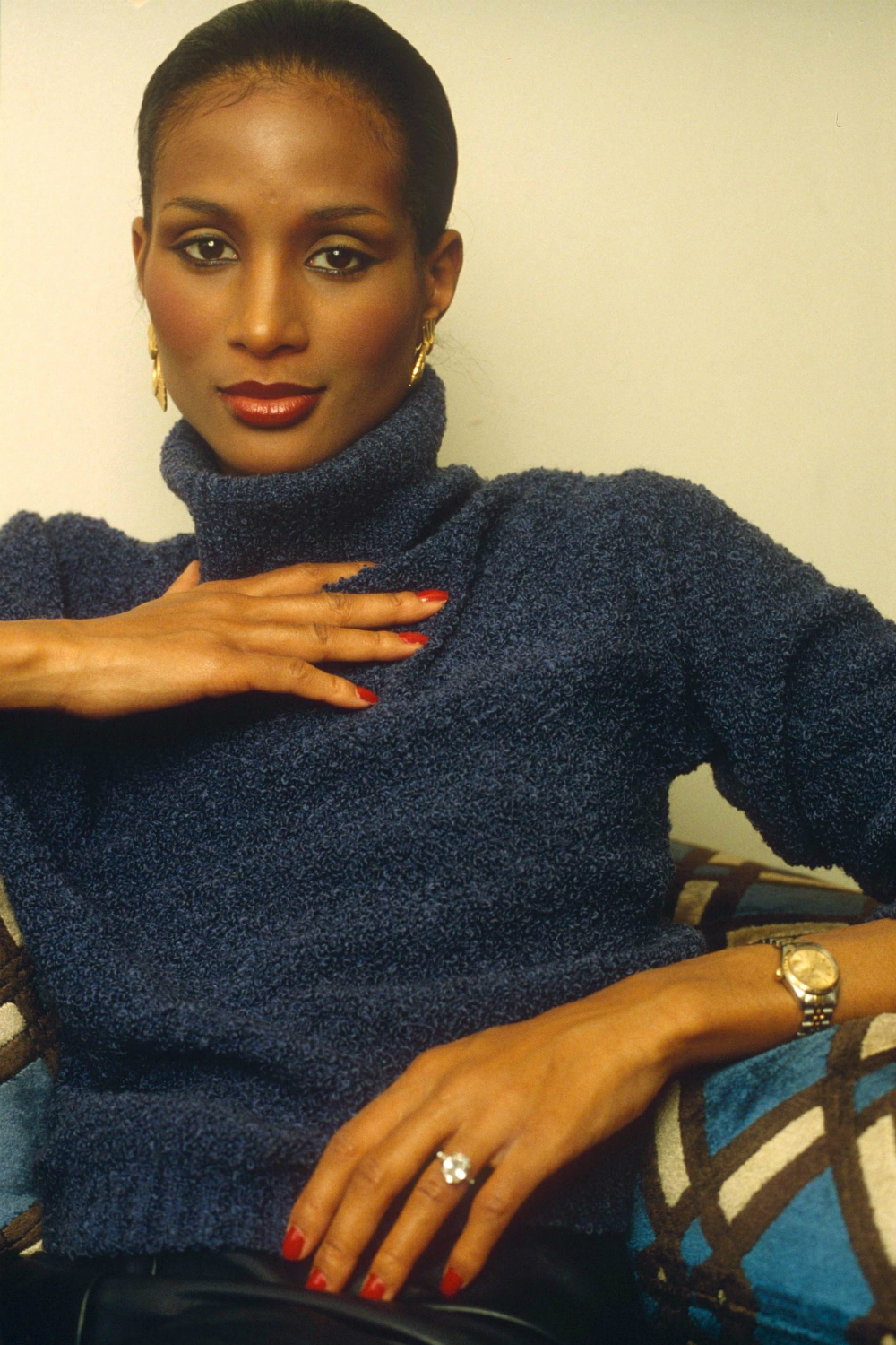
Era: 1970s
From: Buffalo, New York
Her look: Chisel-jawed glamour
USP: Credited with forcing fashion to take black women seriously, she was the first African-American model to appear on the cover of US Vogue in 1974 and ditto French Elle in 1975. Also an actress, she’s appeared in everything from Law & Order to Sabrina, the Teenage Witch in recent years
9. Christie Brinkley
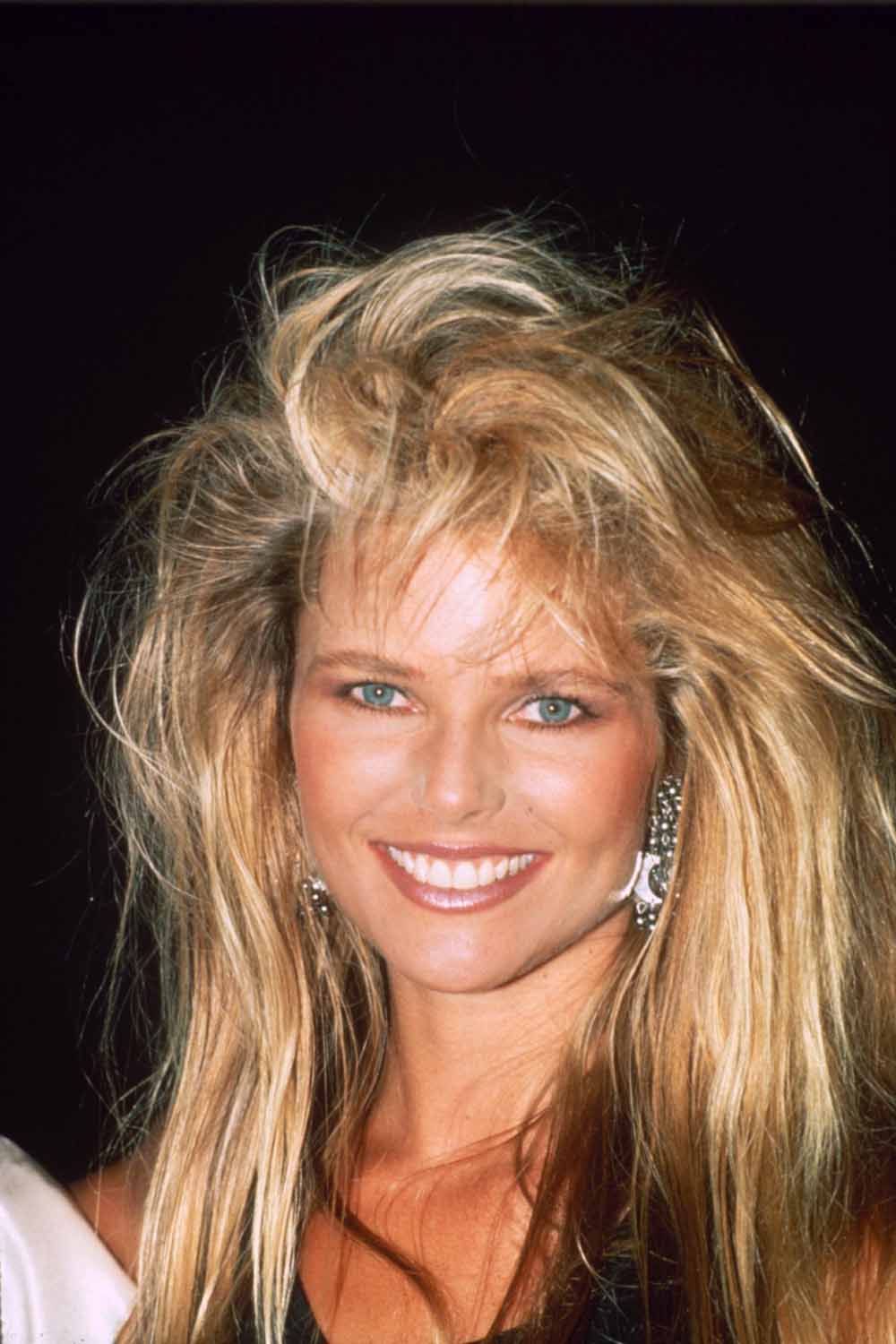
(Image credit: REX/Shutterstock)
Era: 1970s and 1980s From: Michigan, USA Her look: Cookie-cutter California Girl personified (she was brought up in LA) — toned and tanned with a perma-grin USP: She had the longest-running beauty contract of any model, ever — 25 years as the face of Cover Girl. Along with 500 magazine covers, including 3 consecutive Sports Illustrated swimwear issue covers — quite the coup in the 1980s. Also: a spell as Mrs Billy Joel.
10. Cindy Crawford
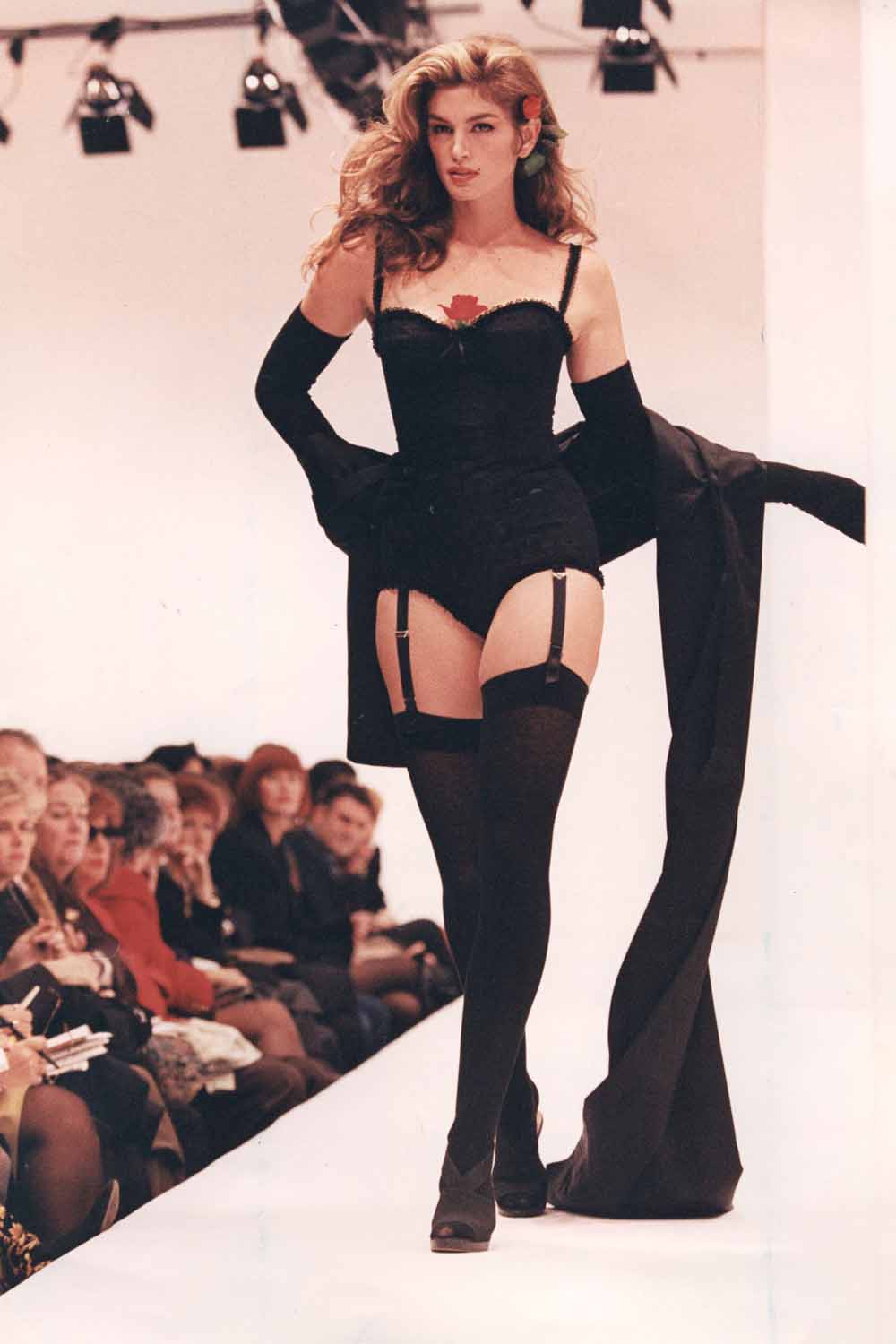
(Image credit: Daily Mail/REX/Shutterstock)
Era: 1980s and 1990s From: Illinois, USA Her look: Big hair, strong brows, athletic body. Hang on, have we forgotten something? Oh yes. The most famous mole OF ALL TIME. USP: Brains and business acumen. She nearly ended up as a chemical engineer and invented the celebrity workout video with her famous ‘Cindy Crawford: Shape Your Body’ exercise series, raking in a fortune in the process.
11. Claudia Schiffer
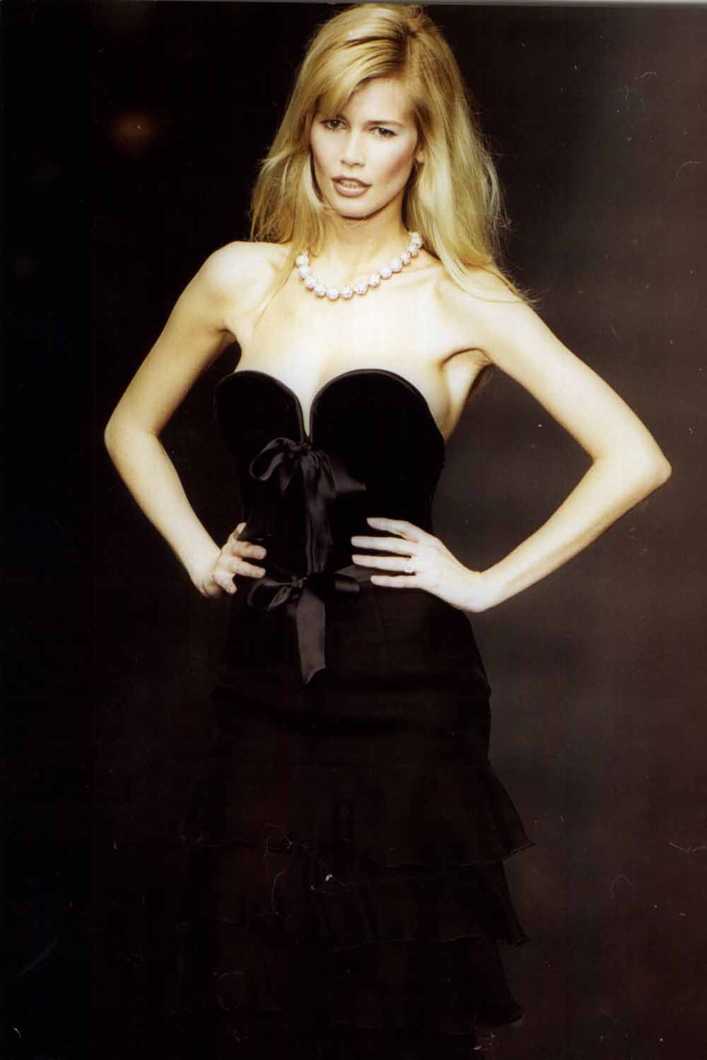
(Image credit: Ken Towner/ANL/REX/Shutterstock)
Era: 1980s and 1990s From: Rheinberg, Germany Her look: Teutonic Brigitte Bardot USP: Holds the world record for most amount of magazine covers, as listed in the Guinness Book of World Records. Was hand-selected by Karl Lagerfeld for his Chanel campaigns and remained one of his favourites for years. But what can top being ‘guillotined’ by permatanned magician David Copperfield (her fiance from 1994-1999) live on stage?
12. Helena Christensen
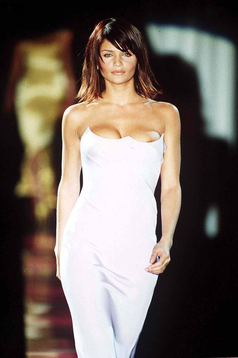
(Image credit: Steve Wood/REX/Shutterstock)
Era: 1980s-present From: Copenhagen, Denmark Her look: Enigmatic and olive-skinned, thanks to her mixed Danish/Peruvian heritage USP: Former Miss Universe Denmark with serious creative skills. She wanted to be a musician and has run her own fashion boutiques (including Butik in New York) and clothing lines. A successful photographer, she was the launch creative director of Nylon magazine, and has held exhibitions of her work
13. Linda Evangelista
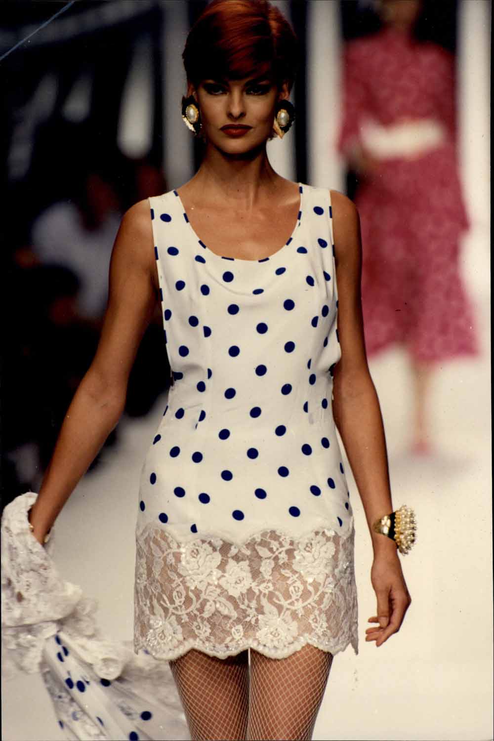
(Image credit: Ken Towner/ANL/REX/Shutterstock)
Era: 1980s-present From: Ontario, Canada Her look: Hawk-nosed chameleon, with ever-changing hair. Long before ‘The Rachel’, it was all about ‘The Linda’ — her 1989 gamine crop that became famous the world over, inspiring wigs and other celebrities (hello, Demi Moore in Ghost). USP: The feisty models’ model. It was she who uttered the infamous phrase, ‘We don’t wake up for less than $10,000 a day,’ referring to her and her fellow supermodel gang. She’s credited with setting a new benchmark for models’ fees and caused controversy by reportedly earning sky-high sums for walking in catwalk shows for the big houses.
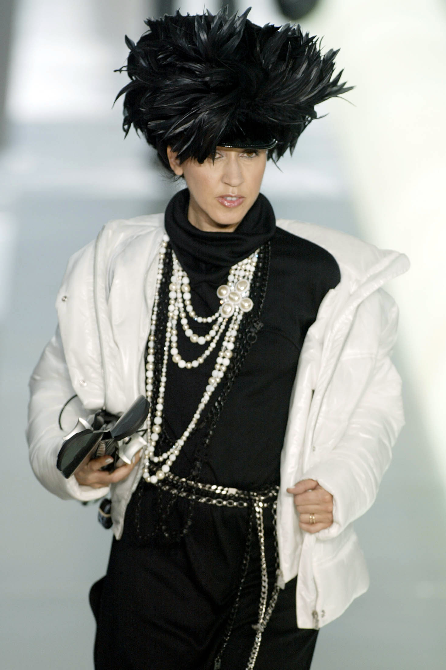
14. Kristen McMenamy
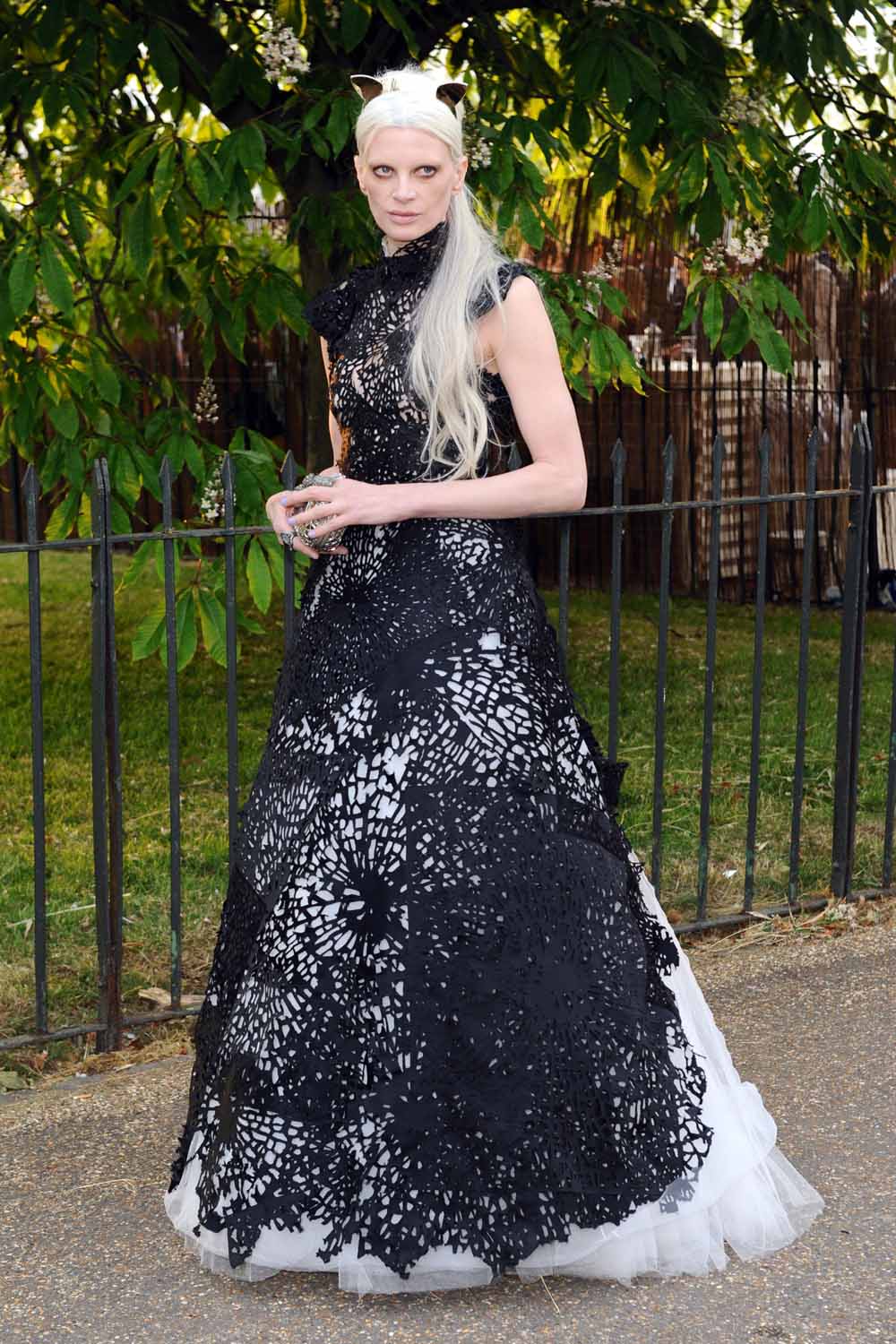
(Image credit: David Fisher/REX/Shutterstock)
Era: 1980s-presentFrom: Pennsylvania, USAHer look: Other-worldly androgynous. Legendary model agent Eileen Ford advised her to have cosmetic surgery — luckily, she pressed on with her unique lookUSP: Ushered in the era of grunge in 1992. Some might say she actually started it, by chopping her long red hair off and letting Francois Nars shave her eyebrows for an Anna Sui catwalk show. Cue international recognition and a starring role in fashion shoots with titles like ‘Grunge & Glory.’ Combined with her theatrical poses and runway ‘walk’, she’s still your go-to girl for high-fashion drama. 15. Christy Turlington
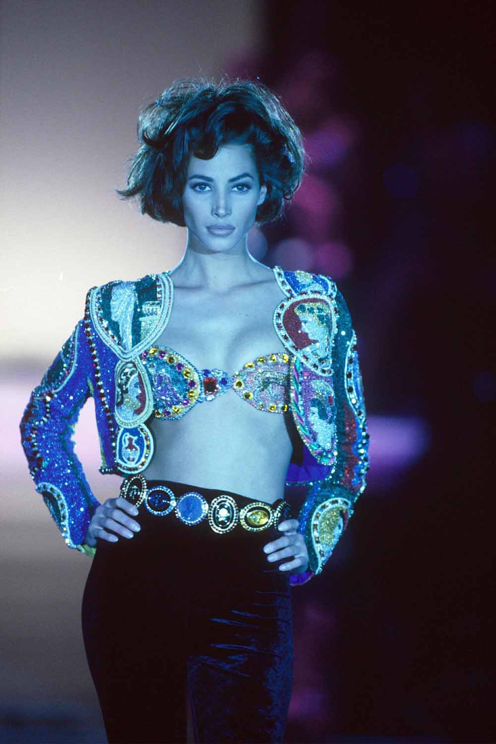
(Image credit: Paul Massey/REX/Shutterstock)
Era: 1980s-present From: California (her mother is from El Salvador), USA Her look: Doe-eyed serenity — the embodiment of Calvin Klein’s fragrance Eternity, one of her most famous campaigns. USP: The Zen One. Having launched her own Ayurvedic skincare line and yoga range, she’s now a prominent campaigner for maternal health in the developing world. She studied for a masters’ degree in public health and launched Every Mother Counts, a non-profit organisation that supports maternal health programmes in countries including Malawi, Uganda, and Indonesia, as well as directing a 2010 documentary on the subject, No Woman, No Cry
16. Elle Macpherson
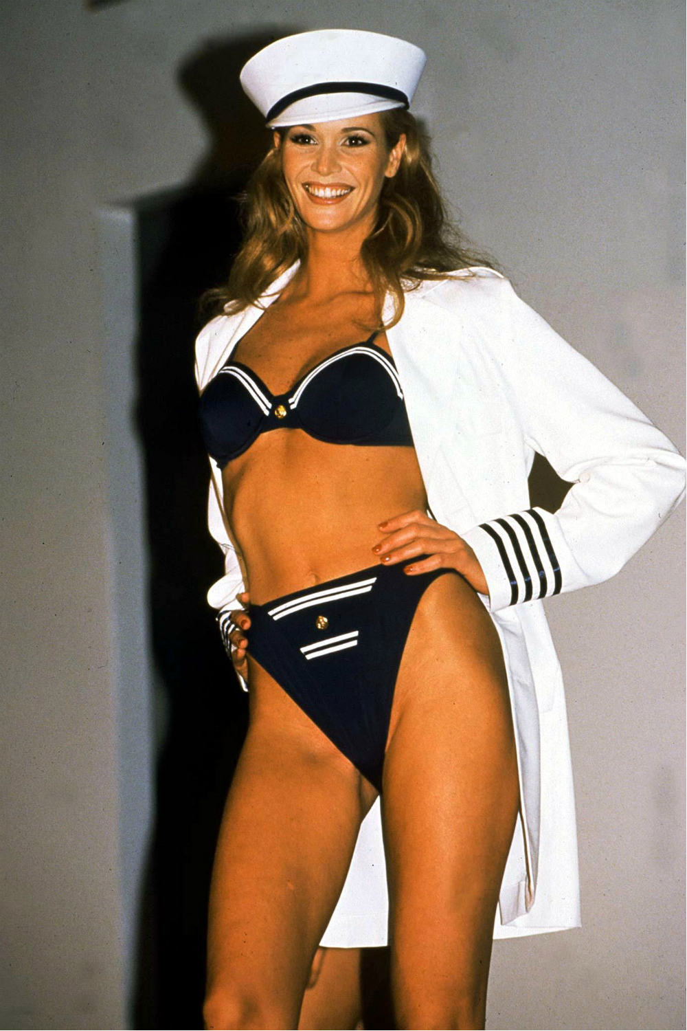
Era: 1980s-present
From: Sydney, Australia
Her Look: Athletic girl-next-door with surfboard abs
USP: She’s graced the cover of a record five Sports Illustrated Swimsuit issues, earning herself the nickname ‘The Body’. She had a ‘Body’-off with Heidi Klum after Klum referred to herself using the same nickname in an advertisement for a Victoria’s Secret bra. Savvy businesswoman to boot, she’s made millions with her lingerie line Elle Macpherson Intimates and was also head judge of Britain & Ireland’s Next Top Model for three years from 2010.
17. Naomi Campbell
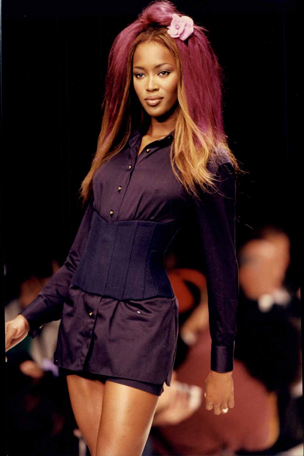
(Image credit: Ken Towner/ANL/REX/Shutterstock)
Era: 1980s-present From: Streatham, South London Her look: Perfectly symmetrical with pillowy pout and serious (some might say ferocious) attitude. USP: Where shall we start? The good: The first black model to appear on the cover of US Vogue’s key September issue (in 1989) Forced the fashion industry to up their bookings of black girls (her pal Yves Saint Laurent threatened to pull his advertising if they didn’t) Starred in a Bob Marley music video at age 7 Took fashion’s most famous tumble on a pair of Vivienne Westwood mega-platforms Was called ‘honorary granddaughter’ by Nelson Mandela Has worked non-stop for charity — including raising £4.5 million (and counting) for disaster relief through her own Fashion For Relief foundation The bad: Um. Convincted of assault four times and accused of various forms of assault or abuse by no less than 9 employees and associates Was forced to appear in a 2010 war crimes trial against former Liberian president Charles Taylor after apparently receiving a ‘blood diamond’ from him. She denied any knowledge.18. Kate Moss
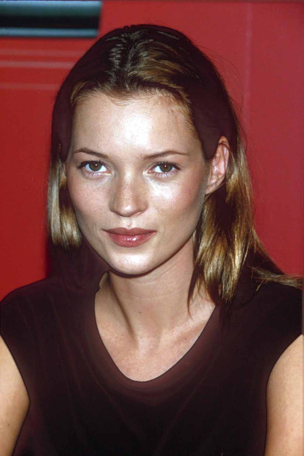
(Image credit: CHARLES SYKES/REX/Shutterstock)
Era: 1980s-present From: Croydon, South London Her look: The Game-Changer: ‘short’ (5’7″), slightly bow-legged, gap-toothed, freckly… The anti-glamazon. USP: The ultimate muse. She rarely speaks, but that’s OK because all other significant cultural voices do it for her. An 18-carat statue of her worth £1.5m created in 2008 for the British Museum was the largest gold statue created since Ancient Egyptian times, a painting of her by Lucian Freud was sold for £3.9 million in 2005, and she’s inspired every fashion photographer from Corinne Day to Mario Testino. Not to mention musicians, including her exes Pete Doherty and Jamie Hince. We won’t start on her actual style. If it wasn’t for her, would ‘Get The Look’ fashion pages even exist?19. Gisele Bundchen
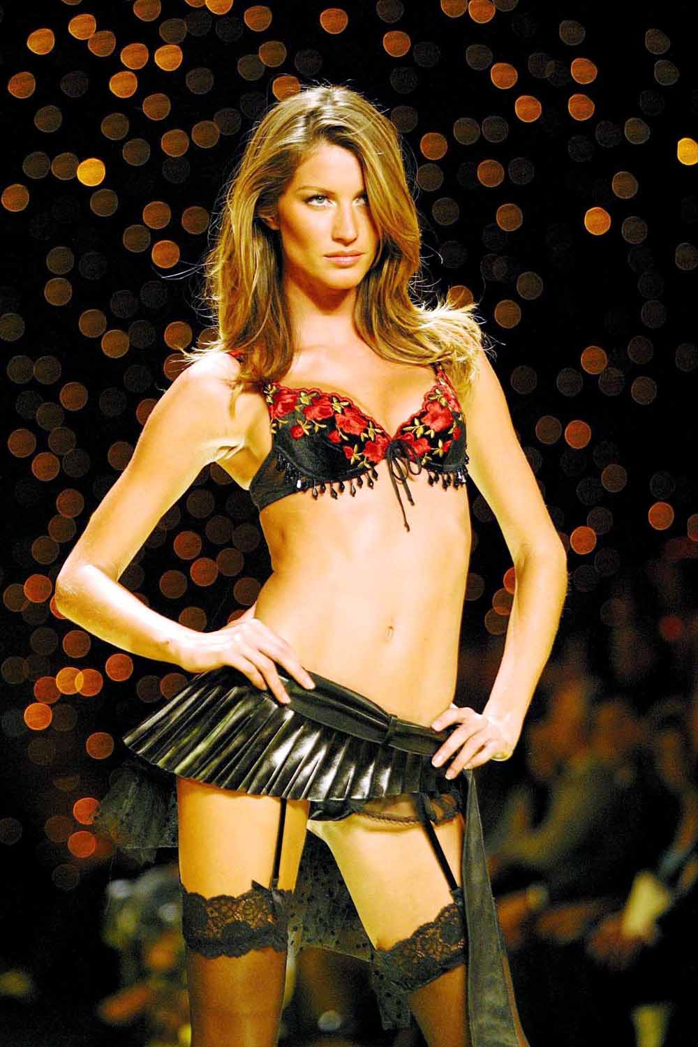
(Image credit: Startraks Photo/REX/Shutterstock)
Era: 1990s-present From: Southern Brazil. Her look: Brazilian bombshell who brought the sexy back. Sunkissed hair, sunkissed limbs, and a special Zoolander-tastic stride known as the ‘horse walk’ — knees up, feet kicking out in front. USP: She’s been the highest-paid model in the world every year since 2004. She wore the most expensive lingerie ever created in the 2000 Victoria’s Secret show (the ‘Red Hot Fantasy Bra’ worth $15 million) and she’s chalked up over 350 ad campaigns and 1,200 magazine covers.
20. Natalia Vodianova

(Image credit: Richard Young/REX/Shutterstock)
Era: 1990s-present From: Gorky, Soviet Union (now Russia) Her look: Dreamy innocent with piercing blue eyes USP: Rags to riches tale following a heartbreaking early start — born into extreme poverty and with a disabled half-sister, she sold fruit on the street as a child to help family finances, before ending up as Viscountess Portman after marrying English property heir Justin Portman. Now goes out with equally illustrious Antoine Arnault, son of LVMH founder Bernard Arnault, and is a mother of four. Yes, four. And she can still shimmy into an Italian sample-size catwalk look 21. Erin O’Connor
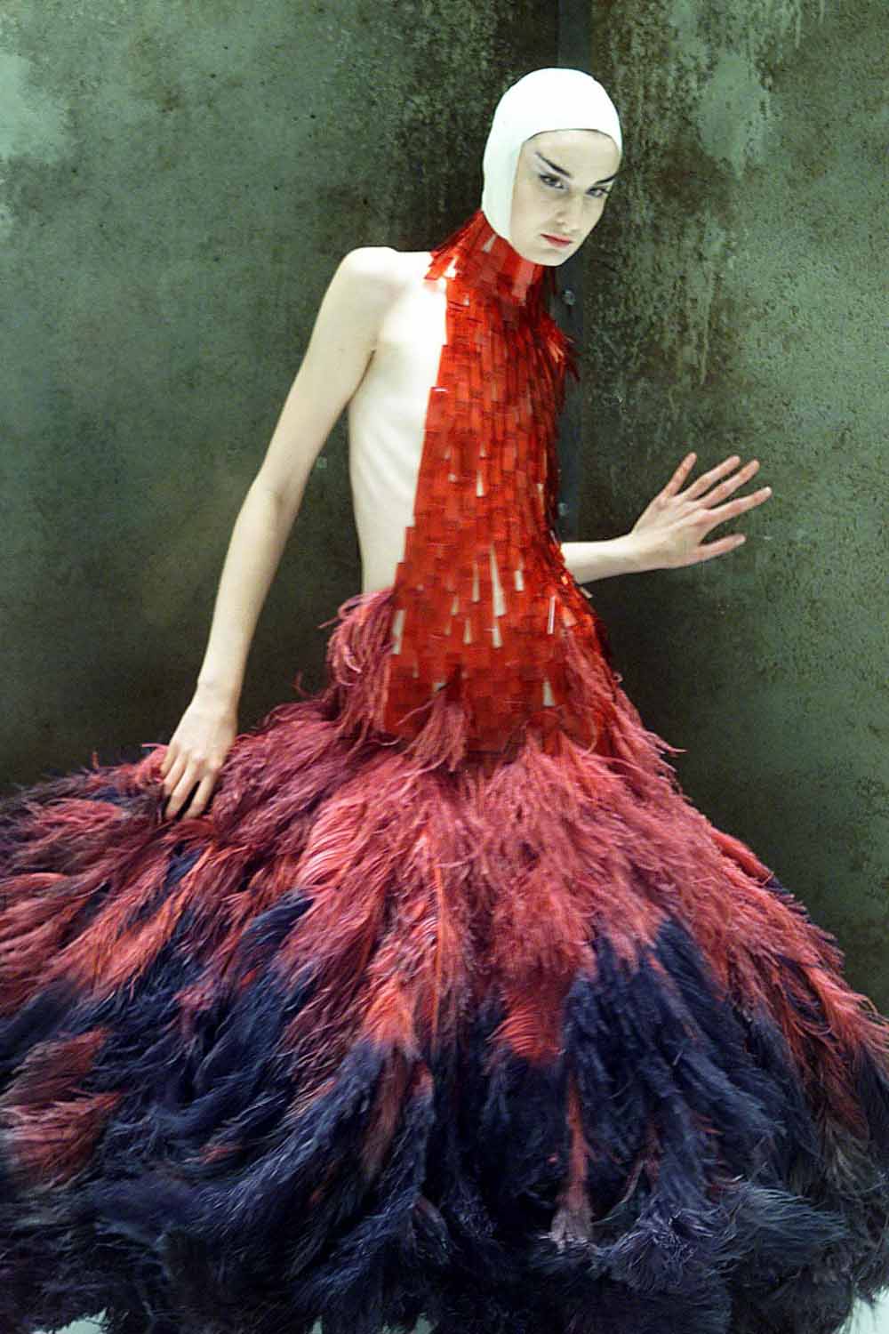
(Image credit: Evening Standar/REX/Shutterstock)
Era: 1990s-present From: West Midlands Her look: Unconventional, angular and aristocratic USP: The favourite muse of fashion’s great creatives, including Alexander McQueen (where she played a madwoman trapped in a glass cage for one of his early shows, Lunatic Asylum), John Galliano and Jean Paul Gaultier, who ‘discovered’ her. One of the few living people to appear on a Royal Mail postage stamp, part of a specially-commissioned set shot by photographer Nick Knight.
22. Alek Wek
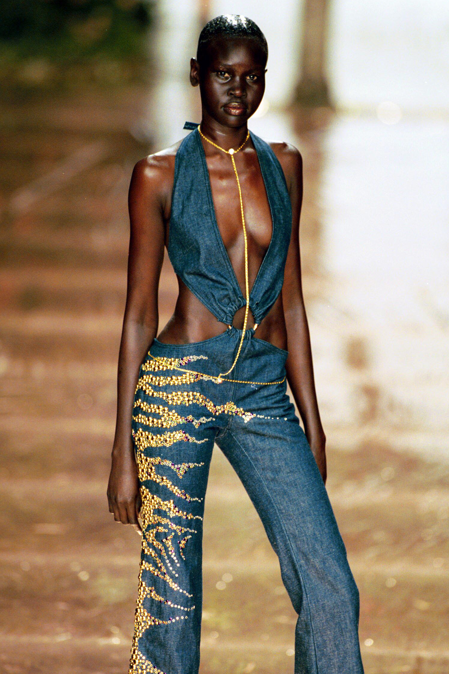
(Image credit: Wood/REX/Shutterstock)
Era: 1995-Present From: Wau, South Sudan Her look: Strong, unique and exotic USP: Dark-skinned models were almost unheard of in the high fashion industry before Wek came along. After being scouted by Models 1 age 14 she became a huge influence on changing beauty ideals and went on to grace the covers of Elle, i-D, Glamour and Cosmopolitan, as well as appearing in editorials for Vogue. She fled her native Sudan in 1991 to escape the civil war and now devotes time to work with UNICEF, Doctors Without Borders and World Vision.
23. Agyness Deyn
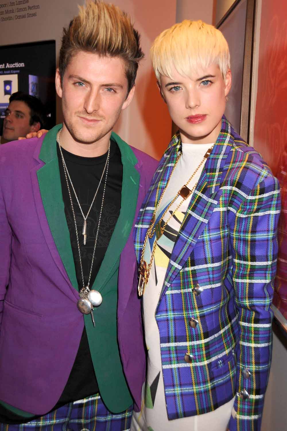
(Image credit: Richard Young/REX/Shutterstock)
Era: 2000s From: Greater Manchester Her look: Punky bleached crop and down-to-earth, non-model ‘walk’. USP: Best mates with teenage pal Henry Holland, it’s fair to say she helped launch his career while he helped launched hers. Her first job was in a chip shop in Rossendale. Now a bona fide serious actress, starring in West End play The Leisure Society and films including Electricity (2013) and Patient Zero (2015)
24. Jessica Stam

(Image credit: Charles Sykes/REX/Shutterstock)
Era: 2000s-present From: Ontario, Canada Her look: Elfin porcelain-doll pretty, with feline eyes USP: She inspired one of the original It bags, the Marc Jacobs ‘Stam’ — a quilted, ladylike frame bag — in 2005. Demand was so high, waiting lists had to be closed. A glammer claim to fame than being the world’s most beautiful dentist — her original career plan. 25. Mariacarla Boscono
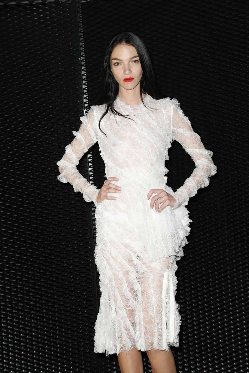
(Image credit: WWD/REX/Shutterstock)
Era: 2000s From: Rome (with a well-travelled childhood featuring spells in Florida, Italy and Kenya) Her look: Black-haired, pale-skinned Sicilian-widow glamour USP: Has appeared in the Pirelli calendar 3 times. She’s earned a place in fashion history as long-running muse to Givenchy’s Riccardo Tisci — she’s basically the human embodiment of his dark, Latin-infused aesthetic.
26. Daria Werbowy
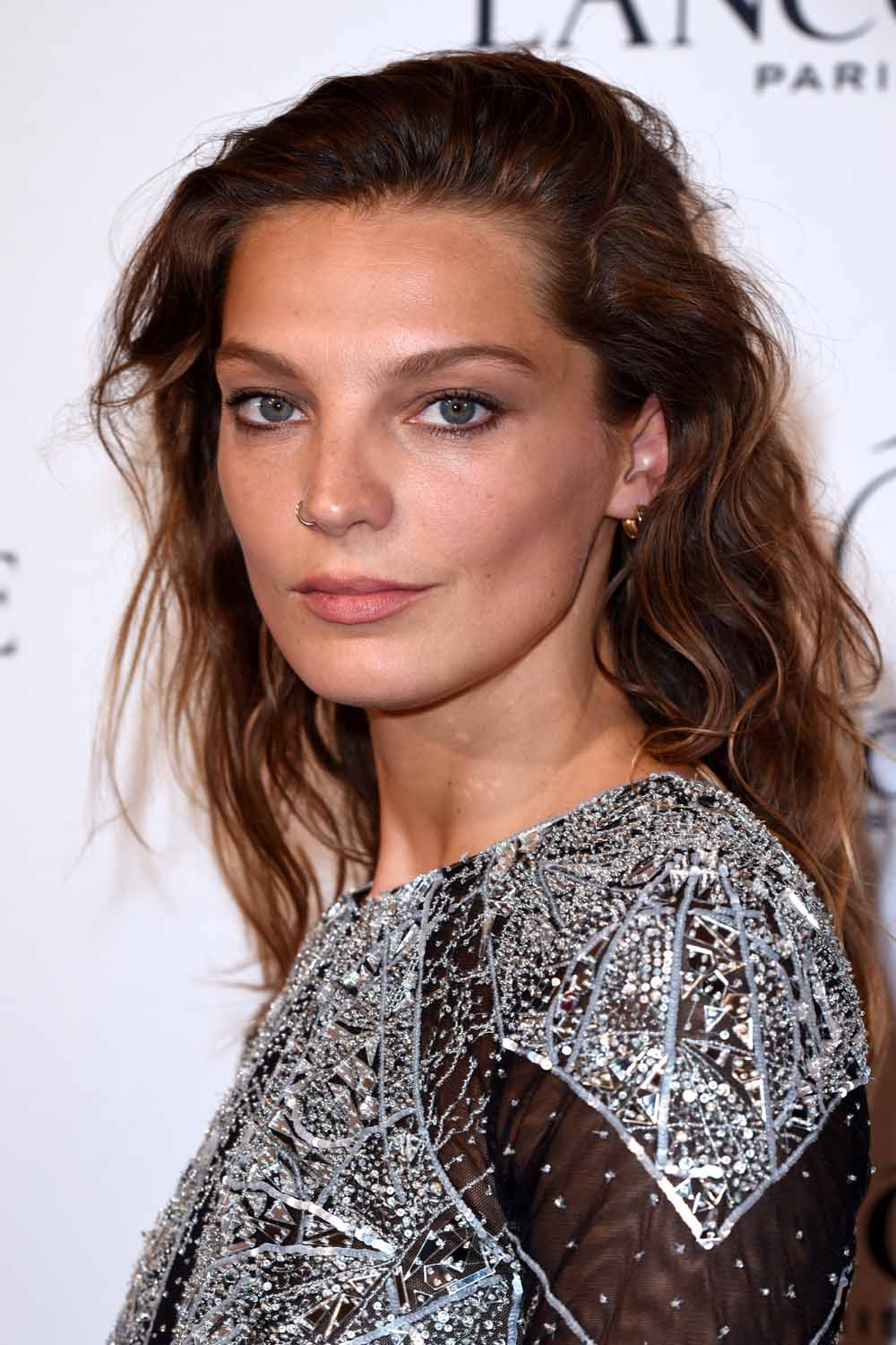
(Image credit: David Fisher/REX/Shutterstock)
Era: 2000s From: Krakow, Poland (she grew up in Canada) Her look: Tawny, leggy, panther-like grace USP: A true fashion models’ model, she holds the all-time record for opening and closing the most shows in a single season. Her long, lithe limbs and cool, natural beauty have been seen in everything from Balmain (the image of her in then-designer Christophe Decarnin’s 2010 collection with its ripped khaki vests, sharp-shouldered military jackets and skinny leather jeans sparked a thousand copycats) to Vogue Paris shoots galore.
27. Liu Wen

Era: 2000s From: Hunan, China
Her look: Delicate features topped off with sweet dimples
USP: Dubbed ‘the first Chinese supermodel’ by reductionists everywhere, it can’t be denied that she’s done a lot to bridge the gap between East and West as far as fashion’s concerned. The first East-Asian model to star in the Victoria’s Secret show, the first East-Asian spokesmodel for Estée Lauder and the first Asian model to make Forbes magazine’s annual highest-paid model ranking. Also riveting: she claims she’s never had a boyfriend. 28. Cara Delevingne

(Image credit: Jim Smeal/BEI/BEI/Shutterstock)
Era: 2010s From: West London Her look: Angel face with beetle brows USP: Aristo with attitude. Impressive array of comedy facial expressions (tongue-out selfie, anyone?) and ‘don’t give a ****’ approach. Her family’s posher than a princess (relatives include a lady-in-waiting to Princess Margaret, baronets and viscounts aplenty and two Lord Mayors of London) but she’s not shy about her undercut or indeed about being bisexual, currently dating female singer St Vincent.29. Edie Campbell
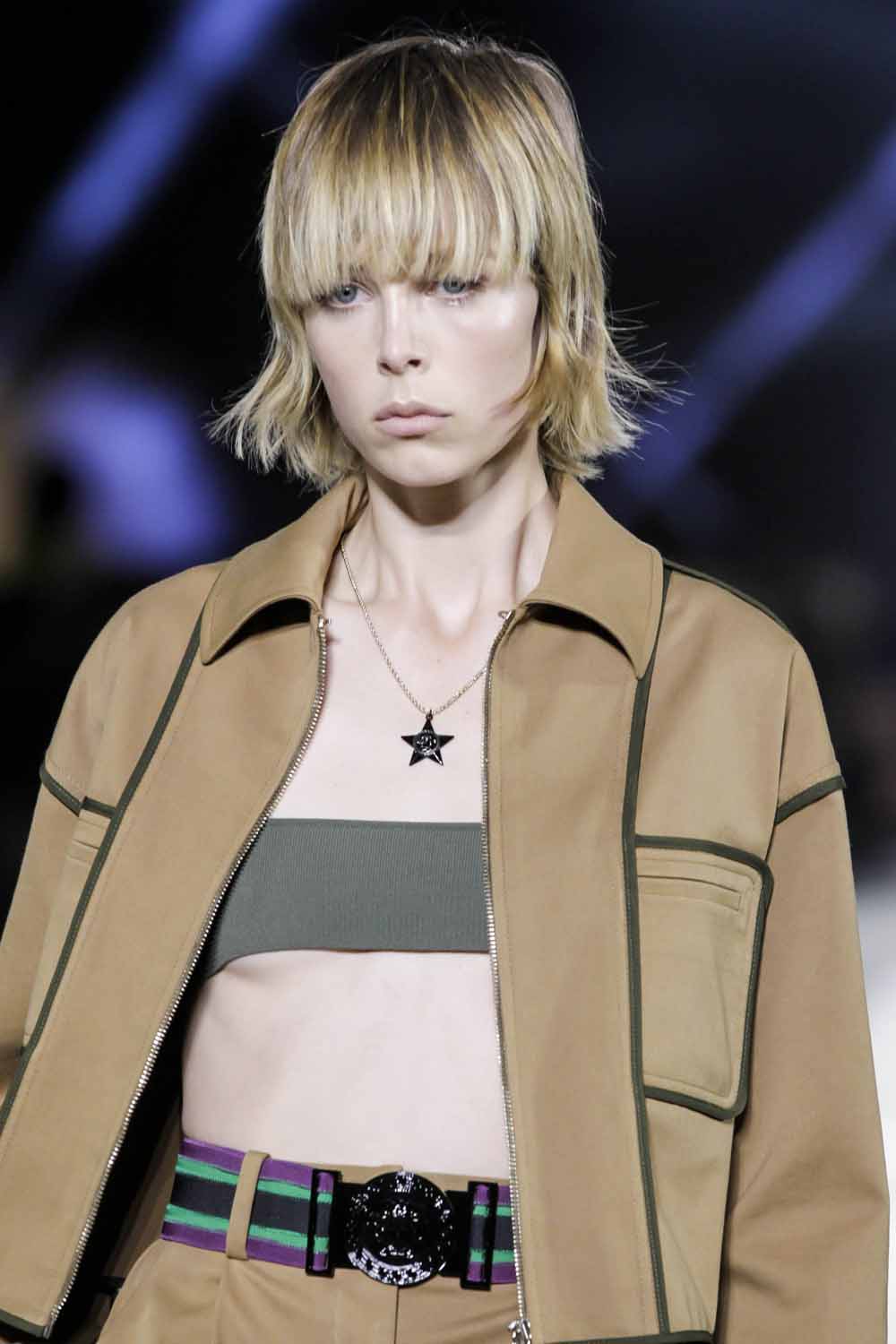
(Image credit: Startraks Photo/REX/Shutterstock)
Era: 2010s From: Westbourne Grove, West London Her look: Unique combo of haughty and kooky — sullen stare, fine features and punky crop USP: A talented jockey, she won the first-ever ladies charity race, The Magnolia Cup, at Goodwood in 2011. No wonder Burberry have snapped her up to convey classy Brit cool personified in ad campaigns galore. 30. Jourdan Dunn
(Image credit: Startraks Photo/REX/Shutterstock)
Era: 2000s-present From: Greenford, West London Her look: Razor-sharp cheekbones and a sultry, sleepy gaze USP: In 2008, she was (sadly) the first black model to walk in a Prada show for over a decade. Now a poster girl for diversity in modelling, causing controversy when she posted on social media that she’d been rejected from a Dior couture show for her boobs and not her skin colour, which she said is what ‘usually happens’. Also a role model for young single mums everywhere — she had her son, Riley, at 19, and has spoken about his battle with sickle-cell anaemia.
31. Kendall Jenner
(Image credit: SIPA/REX/Shutterstock)
Era: 2010s-present From: LA Her look: High-fashion version of the Kardashian LookTM USP: When you book Kendall, you book access to 35 MILLION devoted social media followers. Yup, she was definitely paying attention when Kris ‘n’ Kim were working out the global domination master plan. Google have named her as the second most-searched-for model in the world, and Adweek claimed she generates $236,000 for a single Tweet. The Instagirl generation has arrived.
Modeling is not an easy thing to do and for somebody who is not really interested in what models do ,I may not even be clear what these models do. Somebody may be wondering what they gain by walking on their toes as people watch them. Somebody like that may not even imagine that some of the models earn more than some of the famous people they know. However, not every model is lucky enough to collect these lots of money as it requires particular attributes to do that. All the same, here are the top 10 highest paid models in 2020.
The model must be able to grab every single opportunity they come across and know how to couple these opportunities with great deals. If the model does these two things in the right way then it may just open both doors and windows for cash to start flowing in. Stories have been told about some models who came from very humble backgrounds but latter become filthy rich just because of modeling. If you have a passion for modeling then I will definitely encourage you to follow your dream. It may not just end up being your full-time job but also well rewarding. I invite you to look at the top ten highest paid models in the whole word. These people are filthy rich!
Table of Contents
- 10. Miranda Kerr
- 8. Candice Swanepoel
- 7. Cara Delevingne
- 6. Rosie Huntington-Whiteley
- 5. Gigi Hadid
- 4. Kendall Jenner
- 3. Karlie Kloss
- 2. Adriana Lima
- 1. Gisele Bündchen
10. Miranda Kerr
-
$6,000,000

At the age of thirty four, this model has managed to secure regular payments of up to six million dollars. I mean so many people spend a lot of hours in offices but still they cannot even imagine such amount of money in their bank accounts. Her high paying contracts with Escada fragrance and Wonderba have seen her appear in this list of top earning models this year. The Australian supper model also happens to own a series of glass ware, a cosmetic line and also Kora organics. By my standards I would say that she is really doing well.
At a tender age of thirteen, Kerr had already got herself into the modeling industry. She also happens to be the first Australian to take part in Victoria’s secret campaign and that was in the year two thousand and seven. The events around the year 1997 that saw her make away with victories at nationwide model search which was organized by Impulse fragrances and Dolly Magazine would be considered the turning point for this model as she got her first break through.
However, her winning did not just come alone, it come with controversies surrounding the effects of modeling and fashion on girls of her age at that time. Other than being featured in this list, Kerr is also ranked among the best most admired women. Among many other things, she is also an author of a self help book and owns Kora Organics which happens to be her own brand of organic skin care. I think if you want to be a model you can use a few tips from her but that is just what I think because inspiration is key, even before you get the tips you have to be inspired.
9. Liu Wen
-
$7,000,000


Now this one is interesting because at some point I thought that for you to earn good money if you are a Chinese then you have to find yourself featured in a kung –fu movie but Liu Wen must have proved me wrong. Anyway I still have to confirm if she is not featured in one of such movies. All that put aside, this model’s face and gorgeous body can tell it all. She has a way of coupling her beauty with steady contracts that always see her smiling her way to the bank.
One of the contracts that has seen featured in this list is the contract with La Perla , a high end clothing brand. In addition to that she also has another contract with Estee Launder. This has made hare one of the highest earning Chinese citizens and a very popular lady in the Chinese fashion model
8. Candice Swanepoel
-
$7,100,000

This is another model who has also managed to appear in the list of the most beautiful women on earth. She is a unique model in that she actually cares for her people and this is evident from the support she gives to Mother2Mother, a charity organization that works towards eradication of HIV among the women and children of Africa. This South African diva has mastered the skill of balancing time between her contracts. She currently has three known contracts. Her contracts with Maxfactor, Biotherm and Victoria Secret seem to be well rewarding.
Her career in modeling began when she was lucky to be adopted by a model scout at the age of fifteen. If you have been keen you will realize that she has appeared in several covers some of which include Lush, GQ, Harper’s Bazaar, I-D, Elle among others. In addition to that she is also not a new face in advertising. She has done advertisements for Christian Dior, Jean Paul Gaultier and Jason Wu just to mention but a few.
7. Cara Delevingne
-
$8,500,000

At number seven is not just a model but also a big name in the film industry. I know many did not expect her to be in this list however, Cara Jocelyn Delevingne with a massive following of over thirty four million people on Instagram may have just found a way to making millions making her one of the biggest earners of the year. If you did not know her well allow be to let you know that she is not just a model but also an actress and a singer too. Her history in modeling is rather interesting. Can you imagine that she actually dropped out of school at the age of ten to go into modeling! It paid off anyway. She has been able to win the model of the year awards not once but twice in the years 2014 and 2012 at the British Fashion Awards.
6. Rosie Huntington-Whiteley
-
$9,000,000

I actually did not believe that modeling can also be inborn until I come across this beautiful English model. She is a perfect example of natural talent. It is this talent that makes her carries home a clean nine million dollars. And did I mention that she is feature among the most beautiful English models and I actually think that is one of the reasons she has gained popularity. You can catch her on Instagram @rosiehw and prove to yourself her lifestyle given what she posts that features high-end living.
5. Gigi Hadid
-
$9,000,000

I am tempted to say that models are at their best when they are are in their twenties. This is another young model who is earning big from the industry. In a normal situation, I would say that nine million dollars is too much money to be earned by a twenty two years old lady. However, because of this model, I am willing to change my stand to accommodate extra ordinary cases like hers. Her deals with Topshop, Tommy Hilfiger, Maybelline and BMW may be attributed to her featuring in this list. Moreover, if you do not know her well then you might just be surprised to know that she also appears in The Top 50 models @ models .com
As if that is not enough, the British Fashion Council in the year two thousand and sixteen saw it wise to name Gigi Hadid the International Model of the Year. I would say that she is very lucky to have what many models out there would wish to have and if it is not luck then I do not know what it is.
4. Kendall Jenner
-
$10,000,000

Did you ever imagine that the most beautiful ladies in the earth are also the highest income earners in the word? I guess your answer is a big no but i want to assure you that you are not alone in this because most people I have come across actually know nothing about modeling. However, those who know and understand modeling would know that beautiful ladies in the modeling industry are also among the millionaire list.
In the word today, Kendall Jenner is ranked not only in the list of highest paid models but also among the most beautiful girls in the planet earth. She is a perfect example of a multitalented model with ballet skill to add to her modeling. She is actually among the few models who posses ballet skills. In fact, I have never heard of any other model with such skills. If you are among the Instagram fans then I guess you already know that she is one of the most followed persons on that social media platform. If you are not already following her then check her @kendallienner.
3. Karlie Kloss
-
$10,000,000

There is also a breed of models that couple modeling with entrepreneurship. Karlie Kloss is just one of them. With an estimate earning of ten million dollars, she manages to secure a third position on the list of the higher paid models. She managed to retain the America’s Secret Angel for four consecutive years from the year two thousand and eleven to the year two thousand and fourteen. Besides, she is also ranked among the most beautiful models in America.
2. Adriana Lima
-
$10,500,000

Lima is the longest running angel in the history of Victoria Secret. She has what many of the models in the world would like to have. She is considered a role model by many beginners in the industry. This did not just come easy, from as early as the year two thousand, she was already the spokes model for a renowned cosmetics company named Maybelline cosmetics, a position that she has been holding since then to date. That is not the only contract that she has managed to keep for such a long period of time. Other companies that she has worked with include Kia Motors Commercials and Super Bowl with which she worked with from the year two thousand and three to the year two thousand and nine.
As a result of holding the record of longest running angel in the history of Victoria Secret, she has come to be popularly known as Victoria’s Secret Angel. The most astonishing part of her story is when she first thought of being a model. You will agree with me that some people up to collage level before they know what they really want to do with their lives. That was not the case with this super model; on the contrary she was able to identify her talent while still in elementary school and if you think she waited to be an adult before starting to grab awards, then you are wrong, she was crowed a beauty pageant while in elementary school, an award that motivated her to be what she is today.
1. Gisele Bündchen
-
$30,500,000

At number one is Gisele Bundchen. This one never seizes to amaze me; in fact it looks like riches decided to follow her to retirement. Despite having retired from the modeling industry, her name can still not miss in the list of the top highest paid models in the world and from the look of things she is set to continue featuring in this list. For the past ten years, she has maintained the top slot in the list of super rich models. As a result, she has been named the QUEEN of Supermodels.
This Brazilian model is not just a model, beyond that; she is a producer and an actress. Her modeling star started to shine in the 1990s and she is also a major contributor to the end of heroin chic modeling era in 1999. To some people she is the only remaining true and original supermodel today. Among her achievements is the invention of the “horse walk”. We cannot also ignore the fact that she was actually part of the Victoria’s Secret Angels from the year two thousand to mid two thousand and seven. She also played a movie role in the Devil Wear Prada (2006) and also Taxi (2004).
Conclusion
Modeling in this century is a profession that many would envy since it is evident that it is well paying. However, it requires a lot of determination and self sacrifice to climb to the top because for you to be at the top, you have to be among the best.
Related
-
Facebook
-
Twitterc
-
Google+
-
Pinterest

UPDATE: We have published the updated research summaries of the Top 6 NLP Language Models Transforming AI in 2023.
The introduction of transfer learning and pretrained language models in natural language processing (NLP) pushed forward the limits of language understanding and generation. Transfer learning and applying transformers to different downstream NLP tasks have become the main trend of the latest research advances.
At the same time, there is a controversy in the NLP community regarding the research value of the huge pretrained language models occupying the leaderboards. While lots of AI experts agree with Anna Rogers’s statement that getting state-of-the-art results just by using more data and computing power is not research news, other NLP opinion leaders point out some positive moments in the current trend, like, for example, the possibility of seeing the fundamental limitations of the current paradigm.
Anyway, the latest improvements in NLP language models seem to be driven not only by the massive boosts in computing capacity but also by the discovery of ingenious ways to lighten models while maintaining high performance.
To help you stay up to date with the latest breakthroughs in language modeling, we’ve summarized research papers featuring the key language models introduced during the last few years.
Subscribe to our AI Research mailing list at the bottom of this article to be alerted when we release new summaries.
If you’d like to skip around, here are the papers we featured:
- BERT: Pre-training of Deep Bidirectional Transformers for Language Understanding
- GPT2: Language Models Are Unsupervised Multitask Learners
- XLNet: Generalized Autoregressive Pretraining for Language Understanding
- RoBERTa: A Robustly Optimized BERT Pretraining Approach
- ALBERT: A Lite BERT for Self-supervised Learning of Language Representations
- T5: Exploring the Limits of Transfer Learning with a Unified Text-to-Text Transformer
- GPT3: Language Models Are Few-Shot Learners
- ELECTRA: Pre-training Text Encoders as Discriminators Rather Than Generators
- DeBERTa: Decoding-enhanced BERT with Disentangled Attention
- PaLM: Scaling Language Modeling with Pathways
Important Pretrained Language Models
1. BERT: Pre-training of Deep Bidirectional Transformers for Language Understanding, by Jacob Devlin, Ming-Wei Chang, Kenton Lee, and Kristina Toutanova
Original Abstract
We introduce a new language representation model called BERT, which stands for Bidirectional Encoder Representations from Transformers. Unlike recent language representation models, BERT is designed to pre-train deep bidirectional representations by jointly conditioning on both left and right context in all layers. As a result, the pre-trained BERT representations can be fine-tuned with just one additional output layer to create state-of-the-art models for a wide range of tasks, such as question answering and language inference, without substantial task-specific architecture modifications.
BERT is conceptually simple and empirically powerful. It obtains new state-of-the-art results on eleven natural language processing tasks, including pushing the GLUE benchmark to 80.4% (7.6% absolute improvement), MultiNLI accuracy to 86.7 (5.6% absolute improvement) and the SQuAD v1.1 question answering Test F1 to 93.2 (1.5% absolute improvement), outperforming human performance by 2.0%.
Our Summary
A Google AI team presents a new cutting-edge model for Natural Language Processing (NLP) – BERT, or Bidirectional Encoder Representations from Transformers. Its design allows the model to consider the context from both the left and the right sides of each word. While being conceptually simple, BERT obtains new state-of-the-art results on eleven NLP tasks, including question answering, named entity recognition and other tasks related to general language understanding.

What’s the core idea of this paper?
- Training a deep bidirectional model by randomly masking a percentage of input tokens – thus, avoiding cycles where words can indirectly “see themselves”.
- Also pre-training a sentence relationship model by building a simple binary classification task to predict whether sentence B immediately follows sentence A, thus allowing BERT to better understand relationships between sentences.
- Training a very big model (24 Transformer blocks, 1024-hidden, 340M parameters) with lots of data (3.3 billion word corpus).
What’s the key achievement?
- Advancing the state-of-the-art for 11 NLP tasks, including:
- getting a GLUE score of 80.4%, which is 7.6% of absolute improvement from the previous best result;
- achieving 93.2% accuracy on SQuAD 1.1 and outperforming human performance by 2%.
- Suggesting a pre-trained model, which doesn’t require any substantial architecture modifications to be applied to specific NLP tasks.
What does the AI community think?
- BERT model marks a new era of NLP.
- In a nutshell, two unsupervised tasks together (“fill in the blank” and “does sentence B comes after sentence A?” ) provide great results for many NLP tasks.
- Pre-training of language models becomes a new standard.
What are future research areas?
- Testing the method on a wider range of tasks.
- Investigating the linguistic phenomena that may or may not be captured by BERT.
What are possible business applications?
- BERT may assist businesses with a wide range of NLP problems, including:
- chatbots for better customer experience;
- analysis of customer reviews;
- the search for relevant information, etc.
Where can you get implementation code?
- Google Research has released an official Github repository with Tensorflow code and pre-trained models for BERT.
- PyTorch implementation of BERT is also available on GitHub.
2. Language Models Are Unsupervised Multitask Learners, by Alec Radford, Jeffrey Wu, Rewon Child, David Luan, Dario Amodei, Ilya Sutskever
Original Abstract
Natural language processing tasks, such as question answering, machine translation, reading comprehension, and summarization, are typically approached with supervised learning on task-specific datasets. We demonstrate that language models begin to learn these tasks without any explicit supervision when trained on a new dataset of millions of webpages called WebText. When conditioned on a document plus questions, the answers generated by the language model reach 55 F1 on the CoQA dataset – matching or exceeding the performance of 3 out of 4 baseline systems without using the 127,000+ training examples. The capacity of the language model is essential to the success of zero-shot task transfer and increasing it improves performance in a log-linear fashion across tasks. Our largest model, GPT-2, is a 1.5B parameter Transformer that achieves state of the art results on 7 out of 8 tested language modeling datasets in a zero-shot setting but still underfits WebText. Samples from the model reflect these improvements and contain coherent paragraphs of text. These findings suggest a promising path towards building language processing systems which learn to perform tasks from their naturally occurring demonstrations.
Our Summary
In this paper, the OpenAI team demonstrates that pre-trained language models can be used to solve downstream tasks without any parameter or architecture modifications. They have trained a very big model, a 1.5B-parameter Transformer, on a large and diverse dataset that contains text scraped from 45 million webpages. The model generates coherent paragraphs of text and achieves promising, competitive or state-of-the-art results on a wide variety of tasks.
What’s the core idea of this paper?
- Training the language model on the large and diverse dataset:
- selecting webpages that have been curated/filtered by humans;
- cleaning and de-duplicating the texts, and removing all Wikipedia documents to minimize overlapping of training and test sets;
- using the resulting WebText dataset with slightly over 8 million documents for a total of 40 GB of text.
- Using a byte-level version of Byte Pair Encoding (BPE) for input representation.
- Building a very big Transformer-based model, GPT-2:
- the largest model includes 1542M parameters and 48 layers;
- the model mainly follows the OpenAI GPT model with few modifications (i.e., expanding vocabulary and context size, modifying initialization etc.).
What’s the key achievement?
- Getting state-of-the-art results on 7 out of 8 tested language modeling datasets.
- Showing quite promising results in commonsense reasoning, question answering, reading comprehension, and translation.
- Generating coherent texts, for example, a news article about the discovery of talking unicorns.
What does the AI community think?
- “The researchers built an interesting dataset, applying now-standard tools and yielding an impressive model.” – Zachary C. Lipton, an assistant professor at Carnegie Mellon University.
What are future research areas?
- Investigating fine-tuning on benchmarks such as decaNLP and GLUE to see whether the huge dataset and capacity of GPT-2 can overcome the inefficiencies of BERT’s unidirectional representations.
What are possible business applications?
- In terms of practical applications, the performance of the GPT-2 model without any fine-tuning is far from usable but it shows a very promising research direction.
Where can you get implementation code?
- Initially, OpenAI decided to release only a smaller version of GPT-2 with 117M parameters. The decision not to release larger models was taken “due to concerns about large language models being used to generate deceptive, biased, or abusive language at scale”.
- In November, OpenAI finally released its largest 1.5B-parameter model. The code is available here.
- Hugging Face has introduced a PyTorch implementation of the initially released GPT-2 model.
3. XLNet: Generalized Autoregressive Pretraining for Language Understanding, by Zhilin Yang, Zihang Dai, Yiming Yang, Jaime Carbonell, Ruslan Salakhutdinov, Quoc V. Le
Original Abstract
With the capability of modeling bidirectional contexts, denoising autoencoding based pretraining like BERT achieves better performance than pretraining approaches based on autoregressive language modeling. However, relying on corrupting the input with masks, BERT neglects dependency between the masked positions and suffers from a pretrain-finetune discrepancy. In light of these pros and cons, we propose XLNet, a generalized autoregressive pretraining method that (1) enables learning bidirectional contexts by maximizing the expected likelihood over all permutations of the factorization order and (2) overcomes the limitations of BERT thanks to its autoregressive formulation. Furthermore, XLNet integrates ideas from Transformer-XL, the state-of-the-art autoregressive model, into pretraining. Empirically, XLNet outperforms BERT on 20 tasks, often by a large margin, and achieves state-of-the-art results on 18 tasks including question answering, natural language inference, sentiment analysis, and document ranking.
Our Summary
The researchers from Carnegie Mellon University and Google have developed a new model, XLNet, for natural language processing (NLP) tasks such as reading comprehension, text classification, sentiment analysis, and others. XLNet is a generalized autoregressive pretraining method that leverages the best of both autoregressive language modeling (e.g., Transformer-XL) and autoencoding (e.g., BERT) while avoiding their limitations. The experiments demonstrate that the new model outperforms both BERT and Transformer-XL and achieves state-of-the-art performance on 18 NLP tasks.

What’s the core idea of this paper?
- XLNet combines the bidirectional capability of BERT with the autoregressive technology of Transformer-XL:
- Like BERT, XLNet uses a bidirectional context, which means it looks at the words before and after a given token to predict what it should be. To this end, XLNet maximizes the expected log-likelihood of a sequence with respect to all possible permutations of the factorization order.
- As an autoregressive language model, XLNet doesn’t rely on data corruption, and thus avoids BERT’s limitations due to masking – i.e., pretrain-finetune discrepancy and the assumption that unmasked tokens are independent of each other.
- To further improve architectural designs for pretraining, XLNet integrates the segment recurrence mechanism and relative encoding scheme of Transformer-XL.
What’s the key achievement?
- XLnet outperforms BERT on 20 tasks, often by a large margin.
- The new model achieves state-of-the-art performance on 18 NLP tasks including question answering, natural language inference, sentiment analysis, and document ranking.
What does the AI community think?
- The paper was accepted for oral presentation at NeurIPS 2019, the leading conference in artificial intelligence.
- “The king is dead. Long live the king. BERT’s reign might be coming to an end. XLNet, a new model by people from CMU and Google outperforms BERT on 20 tasks.” – Sebastian Ruder, a research scientist at Deepmind.
- “XLNet will probably be an important tool for any NLP practitioner for a while…[it is] the latest cutting-edge technique in NLP.” – Keita Kurita, Carnegie Mellon University.
What are future research areas?
- Extending XLNet to new areas, such as computer vision and reinforcement learning.
What are possible business applications?
- XLNet may assist businesses with a wide range of NLP problems, including:
- chatbots for first-line customer support or answering product inquiries;
- sentiment analysis for gauging brand awareness and perception based on customer reviews and social media;
- the search for relevant information in document bases or online, etc.
Where can you get implementation code?
- The authors have released the official Tensorflow implementation of XLNet.
- PyTorch implementation of the model is also available on GitHub.
4. RoBERTa: A Robustly Optimized BERT Pretraining Approach, by Yinhan Liu, Myle Ott, Naman Goyal, Jingfei Du, Mandar Joshi, Danqi Chen, Omer Levy, Mike Lewis, Luke Zettlemoyer, Veselin Stoyanov
Original Abstract
Language model pretraining has led to significant performance gains but careful comparison between different approaches is challenging. Training is computationally expensive, often done on private datasets of different sizes, and, as we will show, hyperparameter choices have significant impact on the final results. We present a replication study of BERT pretraining (Devlin et al., 2019) that carefully measures the impact of many key hyperparameters and training data size. We find that BERT was significantly undertrained, and can match or exceed the performance of every model published after it. Our best model achieves state-of-the-art results on GLUE, RACE and SQuAD. These results highlight the importance of previously overlooked design choices, and raise questions about the source of recently reported improvements. We release our models and code.
Our Summary
Natural language processing models have made significant advances thanks to the introduction of pretraining methods, but the computational expense of training has made replication and fine-tuning parameters difficult. In this study, Facebook AI and the University of Washington researchers analyzed the training of Google’s Bidirectional Encoder Representations from Transformers (BERT) model and identified several changes to the training procedure that enhance its performance. Specifically, the researchers used a new, larger dataset for training, trained the model over far more iterations, and removed the next sequence prediction training objective. The resulting optimized model, RoBERTa (Robustly Optimized BERT Approach), matched the scores of the recently introduced XLNet model on the GLUE benchmark.
What’s the core idea of this paper?
- The Facebook AI research team found that BERT was significantly undertrained and suggested an improved recipe for its training, called RoBERTa:
- More data: 160GB of text instead of the 16GB dataset originally used to train BERT.
- Longer training: increasing the number of iterations from 100K to 300K and then further to 500K.
- Larger batches: 8K instead of 256 in the original BERT base model.
- Larger byte-level BPE vocabulary with 50K subword units instead of character-level BPE vocabulary of size 30K.
- Removing the next sequence prediction objective from the training procedure.
- Dynamically changing the masking pattern applied to the training data.
What’s the key achievement?
- RoBERTa outperforms BERT in all individual tasks on the General Language Understanding Evaluation (GLUE) benchmark.
- The new model matches the recently introduced XLNet model on the GLUE benchmark and sets a new state of the art in four out of nine individual tasks.
What are future research areas?
- Incorporating more sophisticated multi-task finetuning procedures.
What are possible business applications?
- Big pretrained language frameworks like RoBERTa can be leveraged in the business setting for a wide range of downstream tasks, including dialogue systems, question answering, document classification, etc.
Where can you get implementation code?
- The models and code used in this study are available on GitHub.
5. ALBERT: A Lite BERT for Self-supervised Learning of Language Representations, by Zhenzhong Lan, Mingda Chen, Sebastian Goodman, Kevin Gimpel, Piyush Sharma, Radu Soricut
Original Abstract
Increasing model size when pretraining natural language representations often results in improved performance on downstream tasks. However, at some point further model increases become harder due to GPU/TPU memory limitations, longer training times, and unexpected model degradation. To address these problems, we present two parameter-reduction techniques to lower memory consumption and increase the training speed of BERT. Comprehensive empirical evidence shows that our proposed methods lead to models that scale much better compared to the original BERT. We also use a self-supervised loss that focuses on modeling inter-sentence coherence, and show it consistently helps downstream tasks with multi-sentence inputs. As a result, our best model establishes new state-of-the-art results on the GLUE, RACE, and SQuAD benchmarks while having fewer parameters compared to BERT-large.
Our Summary
The Google Research team addresses the problem of the continuously growing size of the pretrained language models, which results in memory limitations, longer training time, and sometimes unexpectedly degraded performance. Specifically, they introduce A Lite BERT (ALBERT) architecture that incorporates two parameter-reduction techniques: factorized embedding parameterization and cross-layer parameter sharing. In addition, the suggested approach includes a self-supervised loss for sentence-order prediction to improve inter-sentence coherence. The experiments demonstrate that the best version of ALBERT sets new state-of-the-art results on GLUE, RACE, and SQuAD benchmarks while having fewer parameters than BERT-large.
What’s the core idea of this paper?
- It is not reasonable to further improve language models by making them larger because of memory limitations of available hardware, longer training times, and unexpected degradation of model performance with the increased number of parameters.
- To address this problem, the researchers introduce the ALBERT architecture that incorporates two parameter-reduction techniques:
- factorized embedding parameterization, where the size of the hidden layers is separated from the size of vocabulary embeddings by decomposing the large vocabulary-embedding matrix into two small matrices;
- cross-layer parameter sharing to prevent the number of parameters from growing with the depth of the network.
- The performance of ALBERT is further improved by introducing the self-supervised loss for sentence-order prediction to address BERT’s limitations with regard to inter-sentence coherence.
What’s the key achievement?
- With the introduced parameter-reduction techniques, the ALBERT configuration with 18× fewer parameters and 1.7× faster training compared to the original BERT-large model achieves only slightly worse performance.
- The much larger ALBERT configuration, which still has fewer parameters than BERT-large, outperforms all of the current state-of-the-art language modes by getting:
- 89.4% accuracy on the RACE benchmark;
- 89.4 score on the GLUE benchmark; and
- An F1 score of 92.2 on the SQuAD 2.0 benchmark.
What does the AI community think?
- The paper has been submitted to ICLR 2020 and is available on the OpenReview forum, where you can see the reviews and comments of NLP experts. The reviewers are mainly very appreciative of the presented paper.
What are future research areas?
- Speeding up training and inference through methods like sparse attention and block attention.
- Further improving the model performance through hard example mining, more efficient model training, and other approaches.
What are possible business applications?
- The ALBERT language model can be leveraged in the business setting to improve performance on a wide range of downstream tasks, including chatbot performance, sentiment analysis, document mining, and text classification.
Where can you get implementation code?
- The original implementation of ALBERT is available on GitHub.
- A TensorFlow implementation of ALBERT is also available here.
- A PyTorch implementation of ALBERT can be found here and here.
6. Exploring the Limits of Transfer Learning with a Unified Text-to-Text Transformer, by Colin Raffel, Noam Shazeer, Adam Roberts, Katherine Lee, Sharan Narang, Michael Matena, Yanqi Zhou, Wei Li, Peter J. Liu
Original Abstract
Transfer learning, where a model is first pre-trained on a data-rich task before being fine-tuned on a downstream task, has emerged as a powerful technique in natural language processing (NLP). The effectiveness of transfer learning has given rise to a diversity of approaches, methodology, and practice. In this paper, we explore the landscape of transfer learning techniques for NLP by introducing a unified framework that converts every language problem into a text-to-text format. Our systematic study compares pre-training objectives, architectures, unlabeled datasets, transfer approaches, and other factors on dozens of language understanding tasks. By combining the insights from our exploration with scale and our new “Colossal Clean Crawled Corpus”, we achieve state-of-the-art results on many benchmarks covering summarization, question answering, text classification, and more. To facilitate future work on transfer learning for NLP, we release our dataset, pre-trained models, and code.
Our Summary
The Google research team suggests a unified approach to transfer learning in NLP with the goal to set a new state of the art in the field. To this end, they propose treating each NLP problem as a “text-to-text” problem. Such a framework allows using the same model, objective, training procedure, and decoding process for different tasks, including summarization, sentiment analysis, question answering, and machine translation. The researchers call their model a Text-to-Text Transfer Transformer (T5) and train it on the large corpus of web-scraped data to get state-of-the-art results on a number of NLP tasks.

What’s the core idea of this paper?
- The paper has several important contributions:
- Providing a comprehensive perspective on where the NLP field stands by exploring and comparing existing techniques.
- Introducing a new approach to transfer learning in NLP by suggesting treating every NLP problem as a text-to-text task:
- The model understands which tasks should be performed thanks to the task-specific prefix added to the original input sentence (e.g., “translate English to German:”, “summarize:”).
- Presenting and releasing a new dataset consisting of hundreds of gigabytes of clean web-scraped English text, the Colossal Clean Crawled Corpus (C4).
- Training a large (up to 11B parameters) model, called Text-to-Text Transfer Transformer (T5) on the C4 dataset.
What’s the key achievement?
- The T5 model with 11 billion parameters achieved state-of-the-art performance on 17 out of 24 tasks considered, including:
- a GLUE score of 89.7 with substantially improved performance on CoLA, RTE, and WNLI tasks;
- an Exact Match score of 90.06 on the SQuAD dataset;
- a SuperGLUE score of 88.9, which is a very significant improvement over the previous state-of-the-art result (84.6) and very close to human performance (89.8);
- a ROUGE-2-F score of 21.55 on the CNN/Daily Mail abstractive summarization task.
What are future research areas?
- Researching the methods to achieve stronger performance with cheaper models.
- Exploring more efficient knowledge extraction techniques.
- Further investigating the language-agnostic models.
What are possible business applications?
- Even though the introduced model has billions of parameters and can be too heavy to be applied in the business setting, the presented ideas can be used to improve the performance on different NLP tasks, including summarization, question answering, and sentiment analysis.
Where can you get implementation code?
- The pretrained models together with the dataset and code are released on GitHub.
7. Language Models are Few-Shot Learners, by Tom B. Brown, Benjamin Mann, Nick Ryder, Melanie Subbiah, Jared Kaplan, Prafulla Dhariwal, Arvind Neelakantan, Pranav Shyam, Girish Sastry, Amanda Askell, Sandhini Agarwal, Ariel Herbert-Voss, Gretchen Krueger, Tom Henighan, Rewon Child, Aditya Ramesh, Daniel M. Ziegler, Jeffrey Wu, Clemens Winter, Christopher Hesse, Mark Chen, Eric Sigler, Mateusz Litwin, Scott Gray, Benjamin Chess, Jack Clark, Christopher Berner, Sam McCandlish, Alec Radford, Ilya Sutskever, Dario Amodei
Original Abstract
Recent work has demonstrated substantial gains on many NLP tasks and benchmarks by pre-training on a large corpus of text followed by fine-tuning on a specific task. While typically task-agnostic in architecture, this method still requires task-specific fine-tuning datasets of thousands or tens of thousands of examples. By contrast, humans can generally perform a new language task from only a few examples or from simple instructions – something which current NLP systems still largely struggle to do. Here we show that scaling up language models greatly improves task-agnostic, few-shot performance, sometimes even reaching competitiveness with prior state-of-the-art fine-tuning approaches. Specifically, we train GPT-3, an autoregressive language model with 175 billion parameters, 10× more than any previous non-sparse language model, and test its performance in the few-shot setting. For all tasks, GPT-3 is applied without any gradient updates or fine-tuning, with tasks and few-shot demonstrations specified purely via text interaction with the model. GPT-3 achieves strong performance on many NLP datasets, including translation, question-answering, and cloze tasks, as well as several tasks that require on-the-fly reasoning or domain adaptation, such as unscrambling words, using a novel word in a sentence, or performing 3-digit arithmetic. At the same time, we also identify some datasets where GPT-3’s few-shot learning still struggles, as well as some datasets where GPT-3 faces methodological issues related to training on large web corpora. Finally, we find that GPT-3 can generate samples of news articles which human evaluators have difficulty distinguishing from articles written by humans. We discuss broader societal impacts of this finding and of GPT-3 in general.
Our Summary
The OpenAI research team draws attention to the fact that the need for a labeled dataset for every new language task limits the applicability of language models. Considering that there is a wide range of possible tasks and it’s often difficult to collect a large labeled training dataset, the researchers suggest an alternative solution, which is scaling up language models to improve task-agnostic few-shot performance. They test their solution by training a 175B-parameter autoregressive language model, called GPT-3, and evaluating its performance on over two dozen NLP tasks. The evaluation under few-shot learning, one-shot learning, and zero-shot learning demonstrates that GPT-3 achieves promising results and even occasionally outperforms the state of the art achieved by fine-tuned models.

What’s the core idea of this paper?
- The GPT-3 model uses the same model and architecture as GPT-2, including the modified initialization, pre-normalization, and reversible tokenization.
- However, in contrast to GPT-2, it uses alternating dense and locally banded sparse attention patterns in the layers of the transformer, as in the Sparse Transformer.
- The model is evaluated in three different settings:
- Few-shot learning, when the model is given a few demonstrations of the task (typically, 10 to 100) at inference time but with no weight updates allowed.
- One-shot learning, when only one demonstration is allowed, together with a natural language description of the task.
- Zero-shot learning, when no demonstrations are allowed and the model has access only to a natural language description of the task.
What’s the key achievement?
- The GPT-3 model without fine-tuning achieves promising results on a number of NLP tasks, and even occasionally surpasses state-of-the-art models that were fine-tuned for that specific task:
- On the CoQA benchmark, 81.5 F1 in the zero-shot setting, 84.0 F1 in the one-shot setting, and 85.0 F1 in the few-shot setting, compared to the 90.7 F1 score achieved by fine-tuned SOTA.
- On the TriviaQA benchmark, 64.3% accuracy in the zero-shot setting, 68.0% in the one-shot setting, and 71.2% in the few-shot setting, surpassing the state of the art (68%) by 3.2%.
- On the LAMBADA dataset, 76.2 % accuracy in the zero-shot setting, 72.5% in the one-shot setting, and 86.4% in the few-shot setting, surpassing the state of the art (68%) by 18%.
- The news articles generated by the 175B-parameter GPT-3 model are hard to distinguish from real ones, according to human evaluations (with accuracy barely above the chance level at ~52%).
What are future research areas?
- Improving pre-training sample efficiency.
- Exploring how few-shot learning works.
- Distillation of large models down to a manageable size for real-world applications.
What does the AI community think?
- “The GPT-3 hype is way too much. It’s impressive (thanks for the nice compliments!) but it still has serious weaknesses and sometimes makes very silly mistakes. AI is going to change the world, but GPT-3 is just a very early glimpse. We have a lot still to figure out.” – Sam Altman, CEO and co-founder of OpenAI.
- “I’m shocked how hard it is to generate text about Muslims from GPT-3 that has nothing to do with violence… or being killed…” – Abubakar Abid, CEO and founder of Gradio.
- “No. GPT-3 fundamentally does not understand the world that it talks about. Increasing corpus further will allow it to generate a more credible pastiche but not fix its fundamental lack of comprehension of the world. Demos of GPT-4 will still require human cherry picking.” – Gary Marcus, CEO and founder of Robust.ai.
- “Extrapolating the spectacular performance of GPT3 into the future suggests that the answer to life, the universe and everything is just 4.398 trillion parameters.” – Geoffrey Hinton, Turing Award winner.
What are possible business applications?
- The model with 175B parameters is hard to apply to real business problems due to its impractical resource requirements, but if the researchers manage to distill this model down to a workable size, it could be applied to a wide range of language tasks, including question answering and ad copy generation.
Where can you get implementation code?
- The code itself is not available, but some dataset statistics together with unconditional, unfiltered 2048-token samples from GPT-3 are released on GitHub.
8. ELECTRA: Pre-training Text Encoders as Discriminators Rather Than Generators, by Kevin Clark, Minh-Thang Luong, Quoc V. Le, Christopher D. Manning
Original Abstract
Masked language modeling (MLM) pre-training methods such as BERT corrupt the input by replacing some tokens with [MASK] and then train a model to reconstruct the original tokens. While they produce good results when transferred to downstream NLP tasks, they generally require large amounts of compute to be effective. As an alternative, we propose a more sample-efficient pre-training task called replaced token detection. Instead of masking the input, our approach corrupts it by replacing some tokens with plausible alternatives sampled from a small generator network. Then, instead of training a model that predicts the original identities of the corrupted tokens, we train a discriminative model that predicts whether each token in the corrupted input was replaced by a generator sample or not. Thorough experiments demonstrate this new pre-training task is more efficient than MLM because the task is defined over all input tokens rather than just the small subset that was masked out. As a result, the contextual representations learned by our approach substantially outperform the ones learned by BERT given the same model size, data, and compute. The gains are particularly strong for small models; for example, we train a model on one GPU for 4 days that outperforms GPT (trained using 30× more compute) on the GLUE natural language understanding benchmark. Our approach also works well at scale, where it performs comparably to RoBERTa and XLNet while using less than 1/4 of their compute and outperforms them when using the same amount of compute.
Our Summary
The pre-training task for popular language models like BERT and XLNet involves masking a small subset of unlabeled input and then training the network to recover this original input. Even though it works quite well, this approach is not particularly data-efficient as it learns from only a small fraction of tokens (typically ~15%). As an alternative, the researchers from Stanford University and Google Brain propose a new pre-training task called replaced token detection. Instead of masking, they suggest replacing some tokens with plausible alternatives generated by a small language model. Then, the pre-trained discriminator is used to predict whether each token is an original or a replacement. As a result, the model learns from all input tokens instead of the small masked fraction, making it much more computationally efficient. The experiments confirm that the introduced approach leads to significantly faster training and higher accuracy on downstream NLP tasks.

What’s the core idea of this paper?
- Pre-training methods that are based on masked language modeling are computationally inefficient as they use only a small fraction of tokens for learning.
- Researchers propose a new pre-training task called replaced token detection, where:
- some tokens are replaced by samples from a small generator network;
- a model is pre-trained as a discriminator to distinguish between original and replaced tokens.
- The introduced approach, called ELECTRA (Efficiently Learning an Encoder that Classifies Token Replacements Accurately):
- enables the model to learn from all input tokens instead of the small masked-out subset;
- is not adversarial, despite the similarity to GAN, as the generator producing tokens for replacement is trained with maximum likelihood.
What’s the key achievement?
- Demonstrating that the discriminative task of distinguishing between real data and challenging negative samples is more efficient than existing generative methods for language representation learning.
- Introducing a model that substantially outperforms state-of-the-art approaches while requiring less pre-training compute:
- ELECTRA-Small gets a GLUE score of 79.9 and outperforms a comparably small BERT model with a score of 75.1 and a much larger GPT model with a score of 78.8.
- An ELECTRA model that performs comparably to XLNet and RoBERTa uses only 25% of their pre-training compute.
- ELECTRA-Large outscores the alternative state-of-the-art models on the GLUE and SQuAD benchmarks while still requiring less pre-training compute.
What does the AI community think?
- The paper was selected for presentation at ICLR 2020, the leading conference in deep learning.
What are possible business applications?
- Because of its computational efficiency, the ELECTRA approach can make the application of pre-trained text encoders more accessible to business practitioners.
Where can you get implementation code?
- The original TensorFlow implementation and pre-trained weights are released on GitHub.
9. DeBERTa: Decoding-enhanced BERT with Disentangled Attention, by Pengcheng He, Xiaodong Liu, Jianfeng Gao, Weizhu Chen
Original Abstract
Recent progress in pre-trained neural language models has significantly improved the performance of many natural language processing (NLP) tasks. In this paper we propose a new model architecture DeBERTa (Decoding-enhanced BERT with disentangled attention) that improves the BERT and RoBERTa models using two novel techniques. The first is the disentangled attention mechanism, where each word is represented using two vectors that encode its content and position, respectively, and the attention weights among words are computed using disentangled matrices on their contents and relative positions, respectively. Second, an enhanced mask decoder is used to incorporate absolute positions in the decoding layer to predict the masked tokens in model pre-training. In addition, a new virtual adversarial training method is used for fine-tuning to improve models’ generalization. We show that these techniques significantly improve the efficiency of model pre-training and the performance of both natural language understanding (NLU) and natural language generation (NLG) downstream tasks. Compared to RoBERTa-Large, a DeBERTa model trained on half of the training data performs consistently better on a wide range of NLP tasks, achieving improvements on MNLI by +0.9% (90.2% vs. 91.1%), on SQuAD v2.0 by +2.3% (88.4% vs. 90.7%) and RACE by +3.6% (83.2% vs. 86.8%). Notably, we scale up DeBERTa by training a larger version that consists of 48 Transform layers with 1.5 billion parameters. The significant performance boost makes the single DeBERTa model surpass the human performance on the SuperGLUE benchmark (Wang et al., 2019a) for the first time in terms of macro-average score (89.9 versus 89.8), and the ensemble DeBERTa model sits atop the SuperGLUE leaderboard as of January 6, 2021, outperforming the human baseline by a decent margin (90.3 versus 89.8).
Our Summary
The authors from Microsoft Research propose DeBERTa, with two main improvements over BERT, namely disentangled attention and an enhanced mask decoder. DeBERTa has two vectors representing a token/word by encoding content and relative position respectively. The self-attention mechanism in DeBERTa processes self-attention of content-to-content, content-to-position, and also position-to-content, while the self-attention in BERT is equivalent to only having the first two components. The authors hypothesize that position-to-content self-attention is also needed to comprehensively model relative positions in a sequence of tokens. Furthermore, DeBERTa is equipped with an enhanced mask decoder, where the absolute position of the token/word is also given to the decoder along with the relative information. A single scaled-up variant of DeBERTa surpasses the human baseline on the SuperGLUE benchmark for the first time. The ensemble DeBERTa is the top-performing method on SuperGLUE at the time of this publication.
What’s the core idea of this paper?
- Disentangled attention: In the original BERT, the content embedding and position embedding are added before self-attention and the self-attention is applied only on the output of content and position vectors. The authors hypothesize that this only accounts for content-to-content self-attention and content-to-position self-attention and that we need position-to-content self-attention as well to model position information completely. DeBERTa has two separate vectors representing content and position and self-attention is calculated between all possible pairs, i.e., content-to-content, content-to-position, position-to-content, and position-to-position. Position-to-position self-attention is trivially 1 all the time and has no information, so it is not computed.
- Enhanced mask decoder: The authors hypothesize that the model needs absolute position information to understand syntactical nuances such as subject-object characterization. So, DeBERTa is provided with absolute position information along with relative position information. The absolute position embedding is provided to the last decoder layer just before the softmax layer, which gives the output.

- Scale-invariant fine-tuning: A virtual adversarial training algorithm called scale-invariant fine-tuning is used as a regularization method to increase generalization. The word embeddings are perturbed to a small extent and trained to produce the same output as they would on non-perturbed word embeddings. The word embedding vectors are normalized to stochastic vectors (where the sum of the elements in a vector is 1) to be invariant to the number of parameters in the model.
What’s the key achievement?
- Compared to the current state-of-the-art method RoBERTa-Large, the DeBERTA model trained on half the training data achieves:
- an improvement of +0.9% in accuracy on MNLI (91.1% vs. 90.2%),
- an improvement of +2.3% in accuracy on SQuAD v2.0 (90.7% vs. 88.4%),
- an improvement of +3.6% in accuracy on RACE (86.8% vs. 83.2%)
- A single scaled-up variant of DeBERTa surpasses the human baseline on the SuperGLUE benchmark for the first time (89.9 vs. 89.8). The ensemble DeBERTa is the top-performing method on SuperGLUE at the time of this publication, outperforming the human baseline by a decent margin (90.3 versus 89.8).
What does the AI community think?
- The paper has been accepted to ICLR 2021, one of the key conferences in deep learning.
What are future research areas?
- Improving pretraining by introducing other useful information, in addition to positions, with the Enhanced Mask Decoder (EMD) framework.
- A more comprehensive study of scale-invariant fine-tuning (SiFT).
What are possible business applications?
- The contextual representations of pretrained language modeling could be used in search, question answering, summarization, virtual assistants, and chatbots, among other tasks.
Where can you get implementation code?
- The implementation of DeBERTa is available on GitHub.
10. PaLM: Scaling Language Modeling with Pathways, by Aakanksha Chowdhery, Sharan Narang, Jacob Devlin, Maarten Bosma, Gaurav Mishra, Adam Roberts, Paul Barham, Hyung Won Chung, Charles Sutton, Sebastian Gehrmann, Parker Schuh, Kensen Shi, Sasha Tsvyashchenko, Joshua Maynez, Abhishek Rao, Parker Barnes, Yi Tay, Noam Shazeer, Vinodkumar Prabhakaran, Emily Reif, Nan Du, Ben Hutchinson, Reiner Pope, James Bradbury, Jacob Austin, Michael Isard, Guy Gur-Ari, Pengcheng Yin, Toju Duke, Anselm Levskaya, Sanjay Ghemawat, Sunipa Dev, Henryk Michalewski, Xavier Garcia, Vedant Misra, Kevin Robinson, Liam Fedus, Denny Zhou, Daphne Ippolito, David Luan, Hyeontaek Lim, Barret Zoph, Alexander Spiridonov, Ryan Sepassi, David Dohan, Shivani Agrawal, Mark Omernick, Andrew M. Dai, Thanumalayan Sankaranarayana Pillai, Marie Pellat, Aitor Lewkowycz, Erica Moreira, Rewon Child, Oleksandr Polozov, Katherine Lee, Zongwei Zhou, Xuezhi Wang, Brennan Saeta, Mark Diaz, Orhan Firat, Michele Catasta, Jason Wei, Kathy Meier-Hellstern, Douglas Eck, Jeff Dean, Slav Petrov, Noah Fiedel
Original Abstract
Large language models have been shown to achieve remarkable performance across a variety of natural language tasks using few-shot learning, which drastically reduces the number of task-specific training examples needed to adapt the model to a particular application. To further our understanding of the impact of scale on few-shot learning, we trained a 540-billion parameter, densely activated, Transformer language model, which we call Pathways Language Model PaLM. We trained PaLM on 6144 TPU v4 chips using Pathways, a new ML system which enables highly efficient training across multiple TPU Pods. We demonstrate continued benefits of scaling by achieving state-of-the-art few-shot learning results on hundreds of language understanding and generation benchmarks. On a number of these tasks, PaLM 540B achieves breakthrough performance, outperforming the finetuned state-of-the-art on a suite of multi-step reasoning tasks, and outperforming average human performance on the recently released BIG-bench benchmark. A significant number of BIG-bench tasks showed discontinuous improvements from model scale, meaning that performance steeply increased as we scaled to our largest model. PaLM also has strong capabilities in multilingual tasks and source code generation, which we demonstrate on a wide array of benchmarks. We additionally provide a comprehensive analysis on bias and toxicity, and study the extent of training data memorization with respect to model scale. Finally, we discuss the ethical considerations related to large language models and discuss potential mitigation strategies.
Our Summary
The Google Research team contributed a lot in the area of pre-trained language models with their BERT, ALBERT, and T5 models. One of their latest contributions is the Pathways Language Model (PaLM), a 540-billion parameter, dense decoder-only Transformer model trained with the Pathways system. The goal of the Pathways system is to orchestrate distributed computation for accelerators. With its help, the team was able to efficiently train a single model across multiple TPU v4 Pods. The experiments on hundreds of language understanding and generation tasks demonstrated that PaLM achieves state-of-the-art few-shot performance across most tasks with breakthrough capabilities demonstrated in language understanding, language generation, reasoning, and code-related tasks.

What’s the core idea of this paper?
- The main idea of the paper is to scale training of a 540-billion parameter language model with the Pathways system:
- The team was using data parallelism at the Pod level across two Cloud TPU v4 Pods while using standard data and model parallelism within each Pod.
- They were able to scale training to 6144 TPU v4 chips, the largest TPU-based system configuration used for training to date.
- The model achieved a training efficiency of 57.8% hardware FLOPs utilization, which, as the authors claim, is the highest yet achieved training efficiency for large language models at this scale.
- The training data for the PaLM model included a combination of English and multilingual datasets containing high-quality web documents, books, Wikipedia, conversations, and GitHub code.
What’s the key achievement?
- Numerous experiments demonstrate that model performance steeply increased as the team scaled to their largest model.
- PaLM 540B achieved breakthrough performance on multiple very difficult tasks:
- Language understanding and generation. The introduced model surpassed the few-shot performance of prior large models on 28 out of 29 tasks that include question-answering tasks, cloze and sentence-completion tasks, in-context reading comprehension tasks, common-sense reasoning tasks, SuperGLUE tasks, and more. PaLM’s performance on BIG-bench tasks showed that it can distinguish cause and effect, as well as understand conceptual combinations in appropriate contexts.
- Reasoning. With 8-shot prompting, PaLM solves 58% of the problems in GSM8K, a benchmark of thousands of challenging grade school level math questions, outperforming the prior top score of 55% achieved by fine-tuning the GPT-3 175B model. PaLM also demonstrates the ability to generate explicit explanations in situations that require a complex combination of multi-step logical inference, world knowledge, and deep language understanding.
- Code generation. PaLM performs on par with the fine-tuned Codex 12B while using 50 times less Python code for training, confirming that large language models transfer learning from both other programming languages and natural language data more effectively.

What are future research areas?
- Combining the scaling capabilities of the Pathways system with novel architectural choices and training schemes.
What are possible business applications?
- Similarly to other recently introduced pre-trained language models, PaLM can be applied in a wide range of downstream tasks, including conversational AI, question answering, machine translation, document classification, ad copy generation, code bug fixing, and more.
Where can you get implementation code?
- So far, there was no official code implementation release for PaLM but it actually uses a standard Transformer model architecture, with some customizations.
- Pytorch implementation of the specific Transformer architecture from PaLM can be accessed on GitHub.
If you like these research summaries, you might be also interested in the following articles:
- 2020’s Top AI & Machine Learning Research Papers
- GPT-3 & Beyond: 10 NLP Research Papers You Should Read
- The Latest Breakthroughs in Conversational AI Agents
- What Every NLP Engineer Needs To Know About Pre-Trained Language Models
Enjoy this article? Sign up for more AI research updates.
We’ll let you know when we release more summary articles like this one.

Contents
- 1 Introduction
- 2 What is Word Embeddings?
- 3 What is Word2Vec Model?
- 4 Word2Vec Architecture
- 4.1 i) Continuous Bag of Words (CBOW) Model
- 4.2 ii) Skip-Gram Model
- 4.3 CBOW vs Skip-Gram Word2Vec Model
- 5 Word2Vec using Gensim Library
- 5.1 Installing Gensim Library
- 6 Working with Pretrained Word2Vec Model in Gensim
- 6.1 i) Download Pre-Trained Weights
- 6.2 ii) Load Libraries
- 6.3 iii) Load Pre-Trained Weights
- 6.4 iv) Checking Vectors of Words
- 6.5 iv) Most Similar Words
- 6.6 v) Word Analogies
- 7 Training Custom Word2Vec Model in Gensim
- 7.1 i) Understanding Syntax of Word2Vec()
- 7.2 ii) Dataset for Custom Training
- 7.3 iii) Loading Libraries
- 7.4 iii) Loading of Dataset
- 7.5 iv) Text Preprocessing
- 7.6 v) Train CBOW Word2Vec Model
- 7.7 v) Train Skip-Gram Word2Vec Model
- 7.8 v) Visualizing Word Embeddings
- 7.8.1 a) Visualize Word Embeddings for CBOW
- 7.8.2 b) Visualize Word Embeddings for Skip-Gram
Introduction
In this article, we will see the tutorial for doing word embeddings with the word2vec model in the Gensim library. We will first understand what is word embeddings and what is word2vec model. Then we will see its two types of architectures namely the Continuous Bag of Words (CBOW) model and Skip Gram model. Finally, we will explain how to use the pre-trained word2vec model and how to train a custom word2vec model in Gensim with your own text corpus. And as a bonus, we will also cover the visualization of our custom word2vec model.
What is Word Embeddings?
Machine learning and deep learning algorithms cannot work with text data directly, hence they need to be converted into numerical representations. In NLP, there are techniques like Bag of Words, Term Frequency, TF-IDF, to convert text into numeric vectors. However, these classical techniques do not represent the semantic relationship relationships between the texts in numeric form.
This is where word embedding comes into play. Word Embeddings are numeric vector representations of text that also maintain the semantic and contextual relationships within the words in the text corpus.
In such representation, the words that have stronger semantic relationships are closer to each other in the vector space. As you can see in the below example, the words Apple and Mango are close to each other as they both have many similar features of being fruit. Similarly, the words King and Queen are close to each other because they are similar in the royal context.
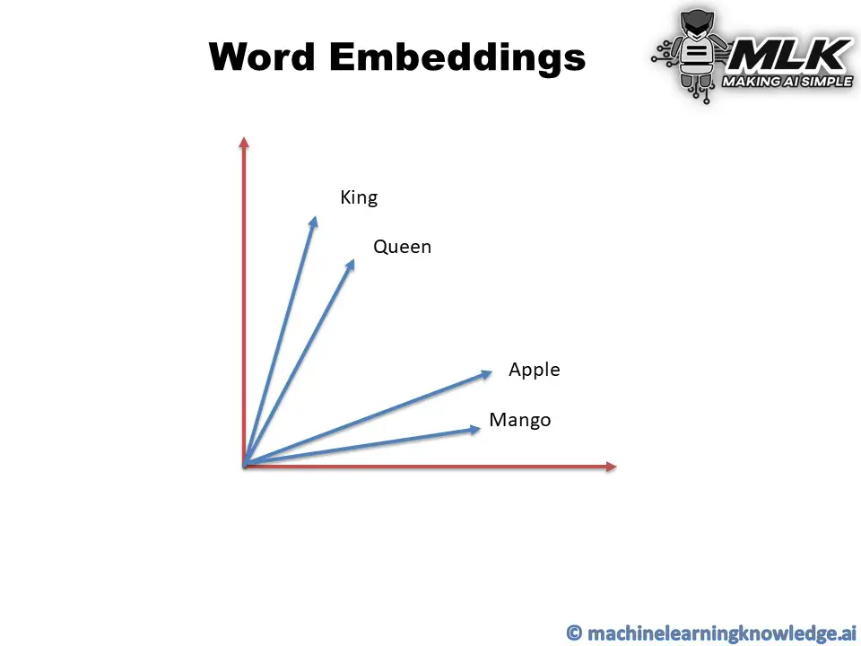
Ad

What is Word2Vec Model?
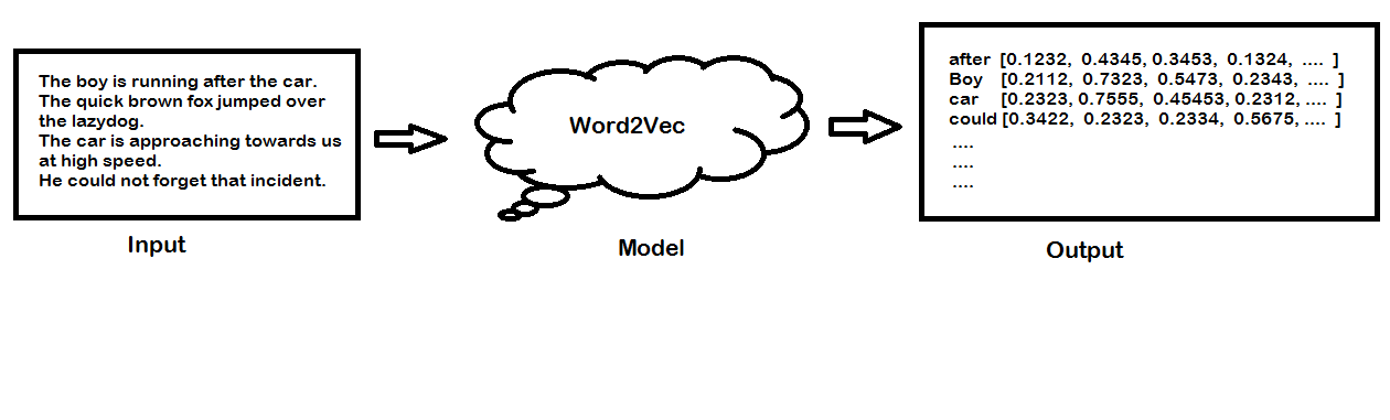
Word2vec is a popular technique for creating word embedding models by using neural network. The word2vec architectures were proposed by a team of researchers led by Tomas Mikolov at Google in 2013.
The word2vec model can create numeric vector representations of words from the training text corpus that maintains the semantic and syntactic relationship. A very famous example of how word2vec preserves the semantics is when you subtract the word Man from King and add Woman it gives you Queen as one of the closest results.
King – Man + Woman ≈ Queen
You may think about how we are doing addition or subtraction with words but do remember that these words are represented by numeric vectors in word2vec so when you apply subtraction and addition the resultant vector is closer to the vector representation of Queen.
In vector space, the word pair of King and Queen and the pair of Man and Woman have similar distances between them. This is another way putting that word2vec can draw the analogy that if Man is to Woman then Kind is to Queen!
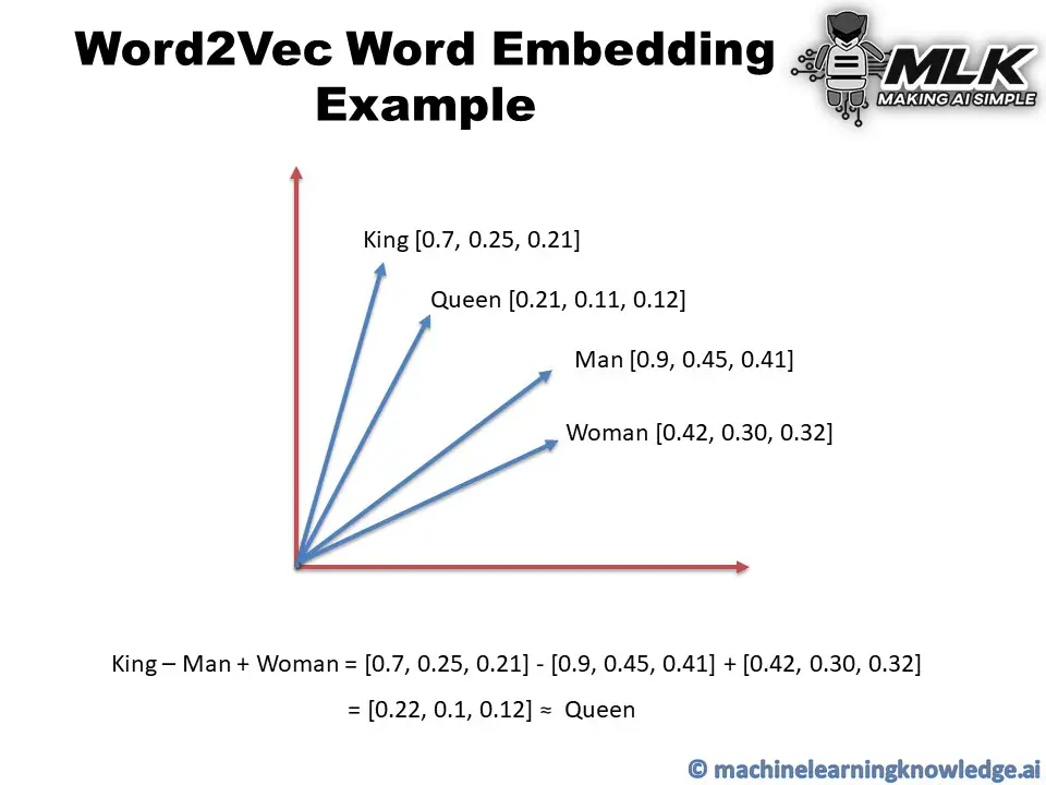
The publicly released model of word2vec by Google consists of 300 features and the model is trained in the Google news dataset. The vocabulary size of the model is around 1.6 billion words. However, this might have taken a huge time for the model to be trained on but they have applied a method of simple subsampling approach to optimize the time.
Word2Vec Architecture
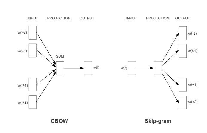
The paper proposed two word2vec architectures to create word embedding models – i) Continuous Bag of Words (CBOW) and ii) Skip-Gram.
i) Continuous Bag of Words (CBOW) Model
In the continuous bag of words architecture, the model predicts the current word from the surrounding context words. The length of the surrounding context word is the window size that is a tunable hyperparameter. The model can be trained by a single hidden layer neural network.
Once the neural network is trained, it results in the vector representation of the words in the training corpus. The size of the vector is also a hyperparameter that we can accordingly choose to produce the best possible results.
ii) Skip-Gram Model
In the skip-gram model, the neural network is trained to predict the surrounding context words given the current word as input. Here also the window size of the surrounding context words is a tunable parameter.
When the neural network is trained, it produces the vector representation of the words in the training corpus. Hera also the size of the vector is a hyperparameter that can be experimented with to produce the best results.
CBOW vs Skip-Gram Word2Vec Model
- CBOW model is trained by predicting the current word by giving the surrounding context words as input. Whereas the Skip-Gram model is trained by predicting the surrounding context words by providing the central word as input.
- CBOW model is faster to train as compared to the Skip-Gram model.
- CBOW model works well to represent the more frequently appearing words whereas Skip-Gram works better to represent less frequent rare words.
For details and information, you may refer to the original word2vec paper here.
Word2Vec using Gensim Library
Gensim is an open-source python library for natural language processing. Working with Word2Vec in Gensim is the easiest option for beginners due to its high-level API for training your own CBOW and SKip-Gram model or running a pre-trained word2vec model.
Installing Gensim Library
Let us install the Gensim library and its supporting library python-Levenshtein.
In[1]:
pip install gensim
pip install python-Levenshtein
In the below sections, we will show you how to run the pre-trained word2vec model in Gensim and then show you how to train your CBOW and SKip-Gram.
(All the examples are shown with Genism 4.0 and may not work with Genism 3.x version)
Working with Pretrained Word2Vec Model in Gensim
i) Download Pre-Trained Weights
We will use the pre-trained weights of word2vec that was trained on Google New corpus containing 3 billion words. This model consists of 300-dimensional vectors for 3 million words and phrases.
The weight can be downloaded from this link. It is a 1.5GB file so make sure you have enough space to save it.
ii) Load Libraries
We load the required Gensim libraries and modules as shown below –
In[2]:
import gensim
from gensim.models import Word2Vec,KeyedVectors
iii) Load Pre-Trained Weights
Next, we load our pre-trained weights by using the KeyedVectors.load_word2vec_format() module of Gensim. Make sure to give the right path of pre-trained weights in the first parameter. (In our case, it is saved in the current working directory)
In[3]:
model = KeyedVectors.load_word2vec_format('GoogleNews-vectors-negative300.bin.gz',binary=True,limit=100000)
iv) Checking Vectors of Words
We can check the numerical vector representation just like the below example where we have shown it for the word man.
In[4]:
vec = model['man']
print(vec)
Out[4]:
[ 0.32617188  0.13085938  0.03466797 -0.08300781  0.08984375 -0.04125977
 -0.19824219  0.00689697  0.14355469  0.0019455   0.02880859 -0.25
 -0.08398438 -0.15136719 -0.10205078  0.04077148 -0.09765625  0.05932617
  0.02978516 -0.10058594 -0.13085938  0.001297    0.02612305 -0.27148438
  0.06396484 -0.19140625 -0.078125    0.25976562  0.375      -0.04541016
  0.16210938  0.13671875 -0.06396484 -0.02062988 -0.09667969  0.25390625
  0.24804688 -0.12695312  0.07177734  0.3203125   0.03149414 -0.03857422
  0.21191406 -0.00811768  0.22265625 -0.13476562 -0.07617188  0.01049805
 -0.05175781  0.03808594 -0.13378906  0.125       0.0559082  -0.18261719
  0.08154297 -0.08447266 -0.07763672 -0.04345703  0.08105469 -0.01092529
  0.17480469  0.30664062 -0.04321289 -0.01416016  0.09082031 -0.00927734
 -0.03442383 -0.11523438  0.12451172 -0.0246582   0.08544922  0.14355469
 -0.27734375  0.03662109 -0.11035156  0.13085938 -0.01721191 -0.08056641
 -0.00708008 -0.02954102  0.30078125 -0.09033203  0.03149414 -0.18652344
 -0.11181641  0.10253906 -0.25976562 -0.02209473  0.16796875 -0.05322266
 -0.14550781 -0.01049805 -0.03039551 -0.03857422  0.11523438 -0.0062561
 -0.13964844  0.08007812  0.06103516 -0.15332031 -0.11132812 -0.14160156
  0.19824219 -0.06933594  0.29296875 -0.16015625  0.20898438  0.00041771
  0.01831055 -0.20214844  0.04760742  0.05810547 -0.0123291  -0.01989746
 -0.00364685 -0.0135498  -0.08251953 -0.03149414  0.00717163  0.20117188
  0.08300781 -0.0480957  -0.26367188 -0.09667969 -0.22558594 -0.09667969
  0.06494141 -0.02502441  0.08496094  0.03198242 -0.07568359 -0.25390625
 -0.11669922 -0.01446533 -0.16015625 -0.00701904 -0.05712891  0.02807617
 -0.09179688  0.25195312  0.24121094  0.06640625  0.12988281  0.17089844
 -0.13671875  0.1875     -0.10009766 -0.04199219 -0.12011719  0.00524902
  0.15625    -0.203125   -0.07128906 -0.06103516  0.01635742  0.18261719
  0.03588867 -0.04248047  0.16796875 -0.15039062 -0.16992188  0.01831055
  0.27734375 -0.01269531 -0.0390625  -0.15429688  0.18457031 -0.07910156
  0.09033203 -0.02709961  0.08251953  0.06738281 -0.16113281 -0.19628906
 -0.15234375 -0.04711914  0.04760742  0.05908203 -0.16894531 -0.14941406
  0.12988281  0.04321289  0.02624512 -0.1796875  -0.19628906  0.06445312
  0.08935547  0.1640625  -0.03808594 -0.09814453 -0.01483154  0.1875
  0.12792969  0.22753906  0.01818848 -0.07958984 -0.11376953 -0.06933594
 -0.15527344 -0.08105469 -0.09277344 -0.11328125 -0.15136719 -0.08007812
 -0.05126953 -0.15332031  0.11669922  0.06835938  0.0324707  -0.33984375
 -0.08154297 -0.08349609  0.04003906  0.04907227 -0.24121094 -0.13476562
 -0.05932617  0.12158203 -0.34179688  0.16503906  0.06176758 -0.18164062
  0.20117188 -0.07714844  0.1640625   0.00402832  0.30273438 -0.10009766
 -0.13671875 -0.05957031  0.0625     -0.21289062 -0.06542969  0.1796875
 -0.07763672 -0.01928711 -0.15039062 -0.00106049  0.03417969  0.03344727
  0.19335938  0.01965332 -0.19921875 -0.10644531  0.01525879  0.00927734
  0.01416016 -0.02392578  0.05883789  0.02368164  0.125       0.04760742
 -0.05566406  0.11572266  0.14746094  0.1015625  -0.07128906 -0.07714844
 -0.12597656  0.0291748   0.09521484 -0.12402344 -0.109375   -0.12890625
  0.16308594  0.28320312 -0.03149414  0.12304688 -0.23242188 -0.09375
 -0.12988281  0.0135498  -0.03881836 -0.08251953  0.00897217  0.16308594
  0.10546875 -0.13867188 -0.16503906 -0.03857422  0.10839844 -0.10498047
  0.06396484  0.38867188 -0.05981445 -0.0612793  -0.10449219 -0.16796875
  0.07177734  0.13964844  0.15527344 -0.03125    -0.20214844 -0.12988281
 -0.10058594 -0.06396484 -0.08349609 -0.30273438 -0.08007812  0.02099609]
iv) Most Similar Words
We can get the list of words similar to the given words by using the most_similar() API of Gensim.
In[5]:
model.most_similar('man')
Out[5]:
[(‘woman’, 0.7664012908935547),
(‘boy’, 0.6824871301651001),
(‘teenager’, 0.6586930155754089),
(‘teenage_girl’, 0.6147903203964233),
(‘girl’, 0.5921714305877686),
(‘robber’, 0.5585119128227234),
(‘teen_ager’, 0.5549196600914001),
(‘men’, 0.5489763021469116),
(‘guy’, 0.5420035123825073),
(‘person’, 0.5342026352882385)]
In[6]:
model.most_similar('PHP')
Out[6]:
[(‘ASP.NET’, 0.7275794744491577),
(‘Visual_Basic’, 0.6807329654693604),
(‘J2EE’, 0.6805503368377686),
(‘Drupal’, 0.6674476265907288),
(‘NET_Framework’, 0.6344218254089355),
(‘Perl’, 0.6339991688728333),
(‘MySQL’, 0.6315538883209229),
(‘AJAX’, 0.6286270618438721),
(‘plugins’, 0.6174636483192444),
(‘SQL’, 0.6123985052108765)]
v) Word Analogies
Let us now see the real working example of King-Man+Woman of word2vec in the below example. After doing this operation we use most_similar() API and can see Queen is at the top of the similarity list.
In[7]:
vec = model['king'] - model['man'] + model['women']
model.most_similar([vec])
Out[7]:
[(‘king’, 0.6478992700576782),
(‘queen’, 0.535493791103363),
(‘women’, 0.5233659148216248),
(‘kings’, 0.5162314772605896),
(‘queens’, 0.4995364248752594),
(‘princes’, 0.46233269572257996),
(‘monarch’, 0.45280295610427856),
(‘monarchy’, 0.4293173849582672),
(‘crown_prince’, 0.42302510142326355),
(‘womens’, 0.41756653785705566)]
Let us see another example, this time we do INR – India + England and amazingly the model returns the currency GBP in the most_similar results.
In[8]:
vec = model['INR'] - model ['India'] + model['England']
model.most_similar([vec])
Out[8]:
[(‘INR’, 0.6442341208457947),
(‘GBP’, 0.5040826797485352),
(‘England’, 0.44649264216423035),
(‘£’, 0.43340998888015747),
(‘Â_£’, 0.4307197630405426),
(‘£_#.##m’, 0.42561301589012146),
(‘GBP##’, 0.42464491724967957),
(‘stg’, 0.42324796319007874),
(‘EUR’, 0.418365478515625),
(‘€’, 0.4151178002357483)]
Training Custom Word2Vec Model in Gensim
i) Understanding Syntax of Word2Vec()
It is very easy to train custom wor2vec model in Gensim with your own text corpus by using Word2Vec() module of gensim.models by providing the following parameters –
- sentences: It is an iterable list of tokenized sentences that will serve as the corpus for training the model.
- min_count: If any word has a frequency below this, it will be ignored.
- workers: Number of CPU worker threads to be used for training the model.
- window: It is the maximum distance between the current and predicted word considered in the sentence during training.
- sg: This denotes the training algorithm. If sg=1 then skip-gram is used for training and if sg=0 then CBOW is used for training.
- epochs: Number of epochs for training.
These are just a few parameters that we are using, but there are many other parameters available for more flexibility. For full syntax check the Gensim documentation here.
ii) Dataset for Custom Training
For the training purpose, we are going to use the first book of the Harry Potter series – “The Philosopher’s Stone”. The text file version can be downloaded from this link.
iii) Loading Libraries
We will be loading the following libraries. TSNE and matplotlib are loaded to visualize the word embeddings of our custom word2vec model.
In[9]:
# For Data Preprocessing
import pandas as pd

# Gensim Libraries
import gensim
from gensim.models import Word2Vec,KeyedVectors

# For visualization of word2vec model
from sklearn.manifold import TSNE
import matplotlib.pyplot as plt
%matplotlib inline
iii) Loading of Dataset
Next, we load the dataset by using the pandas read_csv function.
In[10]:
df = pd.read_csv('HarryPotter.txt', delimiter = "n",header=None)
df.columns = ['Line']
df
Out[10]:
| Line | |
|---|---|
| 0 | / |
| 1 | THE BOY WHO LIVED |
| 2 | Mr. and Mrs. Dursley, of number four, Privet D… |
| 3 | were proud to say that they were perfectly nor… |
| 4 | thank you very much. They were the last people… |
| … | … |
| 6757 | “Oh, I will,” said Harry, and they were surpri… |
| 6758 | the grin that was spreading over his face. “ T… |
| 6759 | know we’re not allowed to use magic at home. I’m |
| 6760 | going to have a lot of fun with Dudley this su… |
| 6761 | Page | 348 |
6762 rows × 1 columns
iv) Text Preprocessing
For preprocessing we are going to use gensim.utils.simple_preprocess that does the basic preprocessing by tokenizing the text corpus into a list of sentences and remove some stopwords and punctuations.
gensim.utils.simple_preprocess module is good for basic purposes but if you are going to create a serious model, we advise using other standard options and techniques for robust text cleaning and preprocessing.
- Also Read – 11 Techniques of Text Preprocessing Using NLTK in Python
In[11]:
preprocessed_text = df['Line'].apply(gensim.utils.simple_preprocess)
preprocessed_text
Out[11]:
0                                                      []
1                                  [the, boy, who, lived]
2       [mr, and, mrs, dursley, of, number, four, priv...
3       [were, proud, to, say, that, they, were, perfe...
4       [thank, you, very, much, they, were, the, last...
                              ...
6757    [oh, will, said, harry, and, they, were, surpr...
6758    [the, grin, that, was, spreading, over, his, f...
6759    [know, we, re, not, allowed, to, use, magic, a...
6760    [going, to, have, lot, of, fun, with, dudley, ...
6761                                               [page]
Name: Line, Length: 6762, dtype: object
v) Train CBOW Word2Vec Model
This is where we train the custom word2vec model with the CBOW technique. For this, we pass the value of sg=0 along with other parameters as shown below.
The value of other parameters is taken with experimentations and may not produce a good model since our goal is to explain the steps for training your own custom CBOW model. You may have to tune these hyperparameters to produce good results.
In[12]:
model_cbow = Word2Vec(sentences=preprocessed_text, sg=0, min_count=10, workers=4, window =3, epochs = 20)
Once the training is complete we can quickly check an example of finding the most similar words to “harry”. It actually does a good job to list out other character’s names that are close friends of Harry Potter. Is it not cool!
In[13]:
model_cbow.wv.most_similar("harry")
Out[13]:
[(‘ron’, 0.8734568953514099),
(‘neville’, 0.8471445441246033),
(‘hermione’, 0.7981335520744324),
(‘hagrid’, 0.7969962954521179),
(‘malfoy’, 0.7925101518630981),
(‘she’, 0.772059977054596),
(‘seamus’, 0.6930352449417114),
(‘quickly’, 0.692932665348053),
(‘he’, 0.691251814365387),
(‘suddenly’, 0.6806278228759766)]
v) Train Skip-Gram Word2Vec Model
For training word2vec with skip-gram technique, we pass the value of sg=1 along with other parameters as shown below. Again, these hyperparameters are just for experimentation and you may like to tune them for better results.
In[14]:
model_skipgram = Word2Vec(sentences =preprocessed_text, sg=1, min_count=10, workers=4, window =10, epochs = 20)
Again, once training is completed, we can check how this model works by finding the most similar words for “harry”. But this time we see the results are not as impressive as the one with CBOW.
In[15]:
model_skipgram.wv.most_similar("harry")
Out[15]:
[(‘goblin’, 0.5757830142974854),
(‘together’, 0.5725131630897522),
(‘shaking’, 0.5482161641120911),
(‘he’, 0.5105234980583191),
(‘working’, 0.5037856698036194),
(‘the’, 0.5015968084335327),
(‘page’, 0.4912668466567993),
(‘story’, 0.4897386431694031),
(‘furiously’, 0.4880291223526001),
(‘then’, 0.47639384865760803)]
v) Visualizing Word Embeddings
The word embedding model created by wor2vec can be visualized by using Matplotlib and the TNSE module of Sklearn. The below code has been referenced from the Kaggle code by Jeff Delaney here and we have just modified the code to make it compatible with Gensim 4.0 version.
In[16]:
def tsne_plot(model):
    "Creates and TSNE model and plots it"
    labels = []
    tokens = []

    for word in model.wv.key_to_index:

        tokens.append(model.wv[word])
        labels.append(word)

    tsne_model = TSNE(perplexity=40, n_components=2, init='pca', n_iter=2500, random_state=23)
    new_values = tsne_model.fit_transform(tokens)

    x = []
    y = []
    for value in new_values:
        x.append(value[0])
        y.append(value[1])

    plt.figure(figsize=(16, 16))
    for i in range(len(x)):
        plt.scatter(x[i],y[i])
        plt.annotate(labels[i],
                     xy=(x[i], y[i]),
                     xytext=(5, 2),
                     textcoords='offset points',
                     ha='right',
                     va='bottom')
    plt.show()
a) Visualize Word Embeddings for CBOW
Let us visualize the word embeddings of our custom CBOW model by using the above custom function.
In[17]:
tsne_plot(model_cbow)
Out[17]:
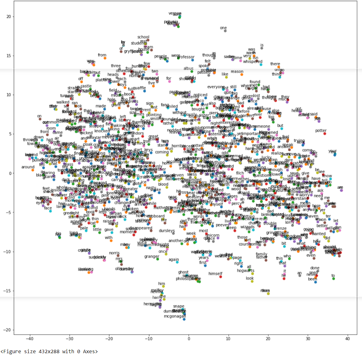
b) Visualize Word Embeddings for Skip-Gram
Let us visualize the word embeddings of our custom Skip-Gram model by using the above custom function.
In[18]:
tsne_plot(model_skipgram)
Out[18]:
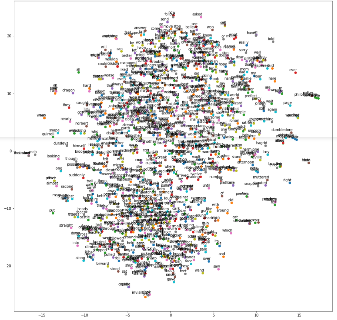
Table of Contents
- What is Transfer Learning
- Word2Vec
- Downloading Google’s word2Vec model
- Support Ticket Classification using Word2Vec
What is Transfer Learning?
Transfer learning is one of the most important breakthroughs in machine learning! It helps us to use the models created by others.
Since everyone doesn’t have access to billions of text snippets and GPU’s/TPU’s to extract patterns from it. If someone can do it and pass on the learnings then we can directly use it and solve business problems.
When someone else creates a model on a huge generic dataset and passes only the model to others for use. This is known as transfer learning because everyone doesn’t have to train the model on such a huge amount of data, hence, they “transfer” the learnings from others to their system.
Transfer learning is really helpful in NLP. Specially vectorization of text, because converting text to vectors for 50K records also is slow. So if we can use the pre-trained models from others, that helps to resolve the problem of converting the text data to numeric data, and we can continue with the other tasks, such as classification or sentiment analysis, etc.
Stanford’s GloVe and Google’s Word2Vec are two really popular choices in Text vectorization using transfer learning.
Word2Vec
Word2vec is not a single algorithm but a combination of two techniques – CBOW(Continuous bag of words) and Skip-gram model.
Both of these are shallow neural networks that map word(s) to the target variable which is also a word(s). Both of these techniques learn weights of the neural network which acts as word vector representations.
Basically each word is represented as a vector of numbers.

CBOW
CBOW(Continuous bag of words) predicts the probability of a word to occur given the words surrounding it. We can consider a single word or a group of words.
Skip-gram model
The Skip-gram model architecture usually tries to achieve the reverse of what the CBOW model does. It tries to predict the source context words (surrounding words) given a target word (the center word)
Which one should be used?
For a large corpus with higher dimensions, it is better to use skip-gram but it is slow to train. Whereas CBOW is better for small corpus and is faster to train too.

Word2Vec vectors are basically a form of word representation that bridges the human understanding of language to that of a machine.
They have learned representations of text in an n-dimensional space where words that have the same meaning have a similar representation. Meaning that two similar words are represented by almost similar vectors(set of numbers) that are very closely placed in a vector space.
For example, look at the below diagram, the words King and Queen appear closer to each other. Similarly, the words Man and Woman appear closer to each other due to the kind of numeric vectors assigned to these words by Word2Vec. If you compute the distance between two words using their numeric vectors, then those words which are related to each other with a context will have less distance between them.
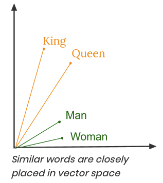
Case Study: Support Ticket Classification using Word2Vec
In a previous case study, I showed you how can you convert Text data into numeric using TF-IDF. And then use it to create a classification model to predict the priority of support tickets.
In this case study, I will use the same dataset and show you how can you use the numeric representations of words from Word2Vec and create a classification model.
Problem Statement: Use the Microsoft support ticket text description to classify a new ticket into P1/P2/P3.
You can download the data required for this case study here.
Reading the support ticket data
This data contains 19,796 rows and 2 columns. The column”body” represents the ticket description and the column “urgency” represents the Priority.
|
import pandas as pd import numpy as np import warnings warnings.filterwarnings(‘ignore’) # Reading the data TicketData=pd.read_csv(‘supportTicketData.csv’) # Printing number of rows and columns print(TicketData.shape) # Printing sample rows TicketData.head(10) |
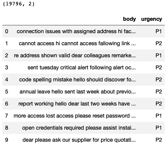
Visualising the distribution of the Target variable
Now we try to see if the Target variable has a balanced distribution or not? Basically each priority type has enough rows to be learned.
If the data would have been imbalanced, for example very less number of rows for the P1 category, then you need to balance the data using any of the popular techniques like over-sampling, under-sampling, or SMOTE.
|
# Number of unique values for urgency column # You can see there are 3 ticket types print(TicketData.groupby(‘urgency’).size()) # Plotting the bar chart %matplotlib inline TicketData.groupby(‘urgency’).size().plot(kind=‘bar’); |

The above bar plot shows that there are enough rows for each ticket type. Hence, this is balanced data for classification.
Count Vectorization: converting text data to numeric
This step will help to remove all the stopwords and create a document term matrix.
We will use this matrix to do further processing. For each word in the document term matrix, we will use the Word2Vec numeric vector representation.
|
1 2 3 4 5 6 7 8 9 10 11 12 13 14 15 16 17 18 19 20 |
# Count vectorization of text from sklearn.feature_extraction.text import CountVectorizer # Ticket Data corpus = TicketData[‘body’].values # Creating the vectorizer vectorizer = CountVectorizer(stop_words=‘english’) # Converting the text to numeric data X = vectorizer.fit_transform(corpus) #print(vectorizer.get_feature_names()) # Preparing Data frame For machine learning # Priority column acts as a target variable and other columns as predictors CountVectorizedData=pd.DataFrame(X.toarray(), columns=vectorizer.get_feature_names()) CountVectorizedData[‘Priority’]=TicketData[‘urgency’] print(CountVectorizedData.shape) CountVectorizedData.head() |
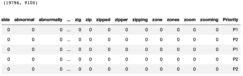
Word2Vec conversion:
Now we will use the Word2Vec representation of words to convert the above document term matrix to a smaller matrix, where the columns are the sum of the vectors for each word present in the document.
For example, look at the below diagram. The flow is shown for one sentence, the same happens for every sentence in the corpus.
- The numeric representation of each word is taken from Word2Vec.
- All the vectors are added, hence producing a single vector
- That single vector represents the information of the sentence, hence treated as one row.

Note: If you feel that your laptop is hanging due to the processing required for the below commands, you can use google colab notebooks!
Downloading Google’s word2Vec model
- We will Use the Pre-trained word2Vec model from google, It contains word vectors for a vocabulary of 3 million words.
- Trained on around 100 billion words from the google news dataset.
Download link: https://drive.google.com/file/d/0B7XkCwpI5KDYNlNUTTlSS21pQmM/edit?usp=sharing
This contains a binary file, that contains numeric representations for each word.
|
#Installing the gensim library required for word2Vec and Doc2Vec !pip install gensim |
|
import gensim #Loading the word vectors from Google trained word2Vec model GoogleModel = gensim.models.KeyedVectors.load_word2vec_format(‘/Users/farukh/Downloads/GoogleNews-vectors-negative300.bin’, binary=True,) |
|
# Each word is a vector of 300 numbers GoogleModel[‘hello’].shape |
![]()
|
# Looking at a sample vector for a word GoogleModel[‘hello’] |

Finding Similar words
This is one of the interesting features of Word2Vec. You can pass a word and find out the most similar words related to the given word.
In the below example, you can see the most relatable word to “king” is “kings” and “queen”. This was possible because of the context learned by the Word2Vec model. Since words like “queen” and “prince” are used in the context of “king”. the numeric word vectors for these words will have similar numbers, hence, the cosine similarity score is high.
|
# Finding similar words # The most_similar() function finds the cosine similarity of the given word with # other words using the word2Vec representations of each word GoogleModel.most_similar(‘king’, topn=5) |

|
# Checking if a word is present in the Model Vocabulary ‘Hello’ in GoogleModel.key_to_index.keys() |
![]()
|
# Creating the list of words which are present in the Document term matrix WordsVocab=CountVectorizedData.columns[:—1] # Printing sample words WordsVocab[0:10] |

Converting every sentence to a numeric vector
For each word in a sentence, we extract the numeric form of the word and then simply add all the numeric forms for that sentence to represent the sentence.
|
1 2 3 4 5 6 7 8 9 10 11 12 13 14 15 16 17 18 19 20 21 22 23 24 |
# Defining a function which takes text input and returns one vector for each sentence def FunctionText2Vec(inpTextData): # Converting the text to numeric data X = vectorizer.transform(inpTextData) CountVecData=pd.DataFrame(X.toarray(), columns=vectorizer.get_feature_names()) # Creating empty dataframe to hold sentences W2Vec_Data=pd.DataFrame() # Looping through each row for the data for i in range(CountVecData.shape[0]): # initiating a sentence with all zeros Sentence = np.zeros(300) # Looping thru each word in the sentence and if its present in # the Word2Vec model then storing its vector for word in WordsVocab[CountVecData.iloc[i , :]>=1]: #print(word) if word in GoogleModel.key_to_index.keys(): Sentence=Sentence+GoogleModel[word] # Appending the sentence to the dataframe W2Vec_Data=W2Vec_Data.append(pd.DataFrame([Sentence])) return(W2Vec_Data) |
|
# Since there are so many words… This will take some time # Calling the function to convert all the text data to Word2Vec Vectors W2Vec_Data=FunctionText2Vec(TicketData[‘body’]) # Checking the new representation for sentences W2Vec_Data.shape |

![]()
|
# Comparing the above with the document term matrix CountVectorizedData.shape |
![]()
Preparing Data for ML
|
# Adding the target variable W2Vec_Data.reset_index(inplace=True, drop=True) W2Vec_Data[‘Priority’]=CountVectorizedData[‘Priority’] # Assigning to DataForML variable DataForML=W2Vec_Data DataForML.head() |

Splitting the data into training and testing
|
# Separate Target Variable and Predictor Variables TargetVariable=DataForML.columns[—1] Predictors=DataForML.columns[:—1] X=DataForML[Predictors].values y=DataForML[TargetVariable].values # Split the data into training and testing set from sklearn.model_selection import train_test_split X_train, X_test, y_train, y_test = train_test_split(X, y, test_size=0.3, random_state=428) # Sanity check for the sampled data print(X_train.shape) print(y_train.shape) print(X_test.shape) print(y_test.shape) |

Standardization/Normalization
This is an optional step. It can speed up the processing of the model training.
|
1 2 3 4 5 6 7 8 9 10 11 12 13 14 15 16 17 18 19 20 21 22 23 |
from sklearn.preprocessing import StandardScaler, MinMaxScaler # Choose either standardization or Normalization # On this data Min Max Normalization is used because we need to fit Naive Bayes # Choose between standardization and MinMAx normalization #PredictorScaler=StandardScaler() PredictorScaler=MinMaxScaler() # Storing the fit object for later reference PredictorScalerFit=PredictorScaler.fit(X) # Generating the standardized values of X X=PredictorScalerFit.transform(X) # Split the data into training and testing set from sklearn.model_selection import train_test_split X_train, X_test, y_train, y_test = train_test_split(X, y, test_size=0.3, random_state=428) # Sanity check for the sampled data print(X_train.shape) print(y_train.shape) print(X_test.shape) print(y_test.shape) |

Training ML classification models
Now the data is ready for machine learning. There are 300-predictors and one target variable. We will use the below algorithms and select the best one out of them based on the accuracy scores you can add more algorithms to this list as per your preferences.
- Naive Bayes
- KNN
- Logistic Regression
- Decision Trees
- AdaBoost
Naive Bayes
This algorithm trains very fast! The accuracy may not be very high always but the speed is guaranteed!
I have commented the cross-validation section just to save computing time. You can uncomment and execute those commands as well.
|
1 2 3 4 5 6 7 8 9 10 11 12 13 14 15 16 17 18 19 20 21 22 23 24 25 26 27 28 29 30 31 |
# Naive Bayes from sklearn.naive_bayes import GaussianNB, MultinomialNB # GaussianNB is used in Binomial Classification # MultinomialNB is used in multi-class classification #clf = GaussianNB() clf = MultinomialNB() # Printing all the parameters of Naive Bayes print(clf) NB=clf.fit(X_train,y_train) prediction=NB.predict(X_test) # Measuring accuracy on Testing Data from sklearn import metrics print(metrics.classification_report(y_test, prediction)) print(metrics.confusion_matrix(y_test, prediction)) # Printing the Overall Accuracy of the model F1_Score=metrics.f1_score(y_test, prediction, average=‘weighted’) print(‘Accuracy of the model on Testing Sample Data:’, round(F1_Score,2)) # Importing cross validation function from sklearn from sklearn.model_selection import cross_val_score # Running 10-Fold Cross validation on a given algorithm # Passing full data X and y because the K-fold will split the data and automatically choose train/test Accuracy_Values=cross_val_score(NB, X , y, cv=5, scoring=‘f1_weighted’) print(‘nAccuracy values for 5-fold Cross Validation:n’,Accuracy_Values) print(‘nFinal Average Accuracy of the model:’, round(Accuracy_Values.mean(),2)) |

KNN
This is a distance-based supervised ML algorithm. Make sure you standardize/normalize the data before using this algorithm, otherwise the accuracy will be low.
|
1 2 3 4 5 6 7 8 9 10 11 12 13 14 15 16 17 18 19 20 21 22 23 24 25 26 27 28 29 30 31 |
# K-Nearest Neighbor(KNN) from sklearn.neighbors import KNeighborsClassifier clf = KNeighborsClassifier(n_neighbors=15) # Printing all the parameters of KNN print(clf) # Creating the model on Training Data KNN=clf.fit(X_train,y_train) prediction=KNN.predict(X_test) # Measuring accuracy on Testing Data from sklearn import metrics print(metrics.classification_report(y_test, prediction)) print(metrics.confusion_matrix(y_test, prediction)) # Printing the Overall Accuracy of the model F1_Score=metrics.f1_score(y_test, prediction, average=‘weighted’) print(‘Accuracy of the model on Testing Sample Data:’, round(F1_Score,2)) # Importing cross validation function from sklearn from sklearn.model_selection import cross_val_score # Running 10-Fold Cross validation on a given algorithm # Passing full data X and y because the K-fold will split the data and automatically choose train/test #Accuracy_Values=cross_val_score(KNN, X , y, cv=10, scoring=’f1_weighted’) #print(‘nAccuracy values for 10-fold Cross Validation:n’,Accuracy_Values) #print(‘nFinal Average Accuracy of the model:’, round(Accuracy_Values.mean(),2)) # Plotting the feature importance for Top 10 most important columns # There is no built-in method to get feature importance in KNN |

Logistic Regression
This algorithm also trains very fast. Hence, whenever we are using high dimensional data, trying out Logistic regression is sensible. The accuracy may not be always the best.
|
1 2 3 4 5 6 7 8 9 10 11 12 13 14 15 16 17 18 19 20 21 22 23 24 25 26 27 28 29 30 31 32 33 34 35 36 37 38 |
# Logistic Regression from sklearn.linear_model import LogisticRegression # choose parameter Penalty=’l1′ or C=1 # choose different values for solver ‘newton-cg’, ‘lbfgs’, ‘liblinear’, ‘sag’, ‘saga’ clf = LogisticRegression(C=10,penalty=‘l2’, solver=‘newton-cg’) # Printing all the parameters of logistic regression # print(clf) # Creating the model on Training Data LOG=clf.fit(X_train,y_train) # Generating predictions on testing data prediction=LOG.predict(X_test) # Printing sample values of prediction in Testing data TestingData=pd.DataFrame(data=X_test, columns=Predictors) TestingData[‘Survived’]=y_test TestingData[‘Predicted_Survived’]=prediction print(TestingData.head()) # Measuring accuracy on Testing Data from sklearn import metrics print(metrics.classification_report(y_test, prediction)) print(metrics.confusion_matrix(prediction, y_test)) ## Printing the Overall Accuracy of the model F1_Score=metrics.f1_score(y_test, prediction, average=‘weighted’) print(‘Accuracy of the model on Testing Sample Data:’, round(F1_Score,2)) ## Importing cross validation function from sklearn #from sklearn.model_selection import cross_val_score ## Running 10-Fold Cross validation on a given algorithm ## Passing full data X and y because the K-fold will split the data and automatically choose train/test #Accuracy_Values=cross_val_score(LOG, X , y, cv=10, scoring=’f1_weighted’) #print(‘nAccuracy values for 10-fold Cross Validation:n’,Accuracy_Values) #print(‘nFinal Average Accuracy of the model:’, round(Accuracy_Values.mean(),2)) |


Decision Tree
This algorithm trains slower as compared to Naive Bayes or Logistic, but it can produce better results.
|
1 2 3 4 5 6 7 8 9 10 11 12 13 14 15 16 17 18 19 20 21 22 23 24 25 26 27 28 29 30 31 32 33 34 |
# Decision Trees from sklearn import tree #choose from different tunable hyper parameters clf = tree.DecisionTreeClassifier(max_depth=20,criterion=‘gini’) # Printing all the parameters of Decision Trees print(clf) # Creating the model on Training Data DTree=clf.fit(X_train,y_train) prediction=DTree.predict(X_test) # Measuring accuracy on Testing Data from sklearn import metrics print(metrics.classification_report(y_test, prediction)) print(metrics.confusion_matrix(y_test, prediction)) # Printing the Overall Accuracy of the model F1_Score=metrics.f1_score(y_test, prediction, average=‘weighted’) print(‘Accuracy of the model on Testing Sample Data:’, round(F1_Score,2)) # Plotting the feature importance for Top 10 most important columns %matplotlib inline feature_importances = pd.Series(DTree.feature_importances_, index=Predictors) feature_importances.nlargest(10).plot(kind=‘barh’) # Importing cross validation function from sklearn #from sklearn.model_selection import cross_val_score # Running 10-Fold Cross validation on a given algorithm # Passing full data X and y because the K-fold will split the data and automatically choose train/test #Accuracy_Values=cross_val_score(DTree, X , y, cv=10, scoring=’f1_weighted’) #print(‘nAccuracy values for 10-fold Cross Validation:n’,Accuracy_Values) #print(‘nFinal Average Accuracy of the model:’, round(Accuracy_Values.mean(),2)) |

Adaboost
This is a tree based boosting algorithm. If the data is not high dimensional, we can use this algorithm. otherwise it takes lot of time to train.
|
1 2 3 4 5 6 7 8 9 10 11 12 13 14 15 16 17 18 19 20 21 22 23 24 25 26 27 28 29 30 31 32 33 34 35 36 37 |
# Adaboost from sklearn.ensemble import AdaBoostClassifier from sklearn.tree import DecisionTreeClassifier # Choosing Decision Tree with 1 level as the weak learner DTC=DecisionTreeClassifier(max_depth=2) clf = AdaBoostClassifier(n_estimators=20, base_estimator=DTC ,learning_rate=0.01) # Printing all the parameters of Adaboost print(clf) # Creating the model on Training Data AB=clf.fit(X_train,y_train) prediction=AB.predict(X_test) # Measuring accuracy on Testing Data from sklearn import metrics print(metrics.classification_report(y_test, prediction)) print(metrics.confusion_matrix(y_test, prediction)) # Printing the Overall Accuracy of the model F1_Score=metrics.f1_score(y_test, prediction, average=‘weighted’) print(‘Accuracy of the model on Testing Sample Data:’, round(F1_Score,2)) # Importing cross validation function from sklearn #from sklearn.model_selection import cross_val_score # Running 10-Fold Cross validation on a given algorithm # Passing full data X and y because the K-fold will split the data and automatically choose train/test #Accuracy_Values=cross_val_score(AB, X , y, cv=10, scoring=’f1_weighted’) #print(‘nAccuracy values for 10-fold Cross Validation:n’,Accuracy_Values) #print(‘nFinal Average Accuracy of the model:’, round(Accuracy_Values.mean(),2)) # Plotting the feature importance for Top 10 most important columns #%matplotlib inline #feature_importances = pd.Series(AB.feature_importances_, index=Predictors) #feature_importances.nlargest(10).plot(kind=’barh’) |

Training the best model on full data
Logistic regression algorithm is producing the highest accuracy on this data, hence, selecting it as final model for deployment.
|
# Generating the Logistic model on full data # This is the best performing model clf = LogisticRegression(C=10,penalty=‘l2’, solver=‘newton-cg’) FinalModel=clf.fit(X,y) |
Making predictions on new cases
To deploy this model, all we need to do is write a function which takes the new data as input, performs all the pre-processing required and passes the data to the Final model.
|
1 2 3 4 5 6 7 8 9 10 11 12 13 14 15 16 17 |
# Defining a function which converts words into numeric vectors for prediction def FunctionPredictUrgency(inpText): # Generating the Glove word vector embeddings X=FunctionText2Vec(inpText) #print(X) # If standardization/normalization was done on training # then the above X must also be converted to same platform # Generating the normalized values of X X=PredictorScalerFit.transform(X) # Generating the prediction using Naive Bayes model and returning Prediction=FinalModel.predict(X) Result=pd.DataFrame(data=inpText, columns=[‘Text’]) Result[‘Prediction’]=Prediction return(Result) |
|
# Calling the function NewTicket=[«help to review the issue», «Please help to resolve system issue»] FunctionPredictUrgency(inpText=NewTicket) |

Conclusion
Transfer learning has made NLP research faster by providing an easy way to share the models produced by big companies and build on top of that. Similar to Word2Vec we have other algorithms like GloVe, Doc2Vec, and BERT which I have discussed in separate case studies.
I hope this post helped you to understand how Word2Vec vectors are created and how to use them to convert any text into numeric form.
Consider sharing this post with your friends to spread the knowledge and help me grow as well! 🙂

Lead Data Scientist
Farukh is an innovator in solving industry problems using Artificial intelligence. His expertise is backed with 10 years of industry experience. Being a senior data scientist he is responsible for designing the AI/ML solution to provide maximum gains for the clients. As a thought leader, his focus is on solving the key business problems of the CPG Industry. He has worked across different domains like Telecom, Insurance, and Logistics. He has worked with global tech leaders including Infosys, IBM, and Persistent systems. His passion to teach inspired him to create this website!